

5.3 Arnol’d Diffusion and Nekhoroshev Time
137
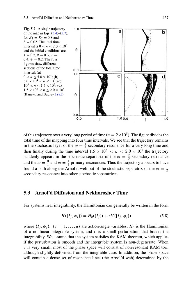
Fig. 5.2 A single trajectory
of the map in Eqs. (5.4)–(5.7),
for K 1 = K 2 = 0.8 and
b = 0.02. The total time
interval is 0 < n < 2.0 × 10 5
and the initial conditions are
I = 0.5, θ = 0.3, J =
0.4, ψ = 0.2. The four
figures show different
sections of the total time
interval: (a)
0 < n ≤ 5.0 × 10 4 ; (b)
5.0 × 10 4 < n ≤ 10 5 ; (c)
10 5 < n ≤ 1.5 × 10 5 ; (d)
1.5 × 10 5 < n ≤ 2.0 × 10 5
(Kaneko and Bagley 1985)
of this trajectory over a very long period of time (n = 2×10 5 ). The figure divides the
total time of the mapping into four time intervals. We see that the trajectory remains
in the stochastic layer of the ω =
1
2 secondary resonance for a very long time and
then finally during the time interval 1.5 × 10 5 < n < 2.0 × 10 5 the trajectory
suddenly appears in the stochastic separatrix of the ω =
2
3 secondary resonance
and the ω =
0
1 and ω =
1
1 primary resonances. Thus the trajectory appears to have
found a path along the Arnol’d web out of the stochastic separatrix of the ω =
1
2
secondary resonance into other stochastic separatrices.
5.3 Arnol’d Diffusion and Nekhoroshev Time
For systems near integrability, the Hamiltonian can generally be written in the form
H ({I j , φ j }) = H 0 ({I j }) + ({I j , φ j })
(5.8)
where {I j , φ j }, (j = 1, . . . , d) are action-angle variables, H 0 is the Hamiltonian
of a nonlinear integrable system, and is a small perturbation that breaks the
integrability. We assume that the system satisfies the KAM theorem, which applies
if the perturbation is smooth and the integrable system is non-degenerate. When
is very small, most of the phase space will consist of non-resonant KAM tori,
although slightly deformed from the integrable case. In addition, the phase space
will contain a dense set of resonance lines (the Arnol’d web) determined by the
137
Fig. 5.2 A single trajectory
of the map in Eqs. (5.4)–(5.7),
for K 1 = K 2 = 0.8 and
b = 0.02. The total time
interval is 0 < n < 2.0 × 10 5
and the initial conditions are
I = 0.5, θ = 0.3, J =
0.4, ψ = 0.2. The four
figures show different
sections of the total time
interval: (a)
0 < n ≤ 5.0 × 10 4 ; (b)
5.0 × 10 4 < n ≤ 10 5 ; (c)
10 5 < n ≤ 1.5 × 10 5 ; (d)
1.5 × 10 5 < n ≤ 2.0 × 10 5
(Kaneko and Bagley 1985)
of this trajectory over a very long period of time (n = 2×10 5 ). The figure divides the
total time of the mapping into four time intervals. We see that the trajectory remains
in the stochastic layer of the ω =
1
2 secondary resonance for a very long time and
then finally during the time interval 1.5 × 10 5 < n < 2.0 × 10 5 the trajectory
suddenly appears in the stochastic separatrix of the ω =
2
3 secondary resonance
and the ω =
0
1 and ω =
1
1 primary resonances. Thus the trajectory appears to have
found a path along the Arnol’d web out of the stochastic separatrix of the ω =
1
2
secondary resonance into other stochastic separatrices.
5.3 Arnol’d Diffusion and Nekhoroshev Time
For systems near integrability, the Hamiltonian can generally be written in the form
H ({I j , φ j }) = H 0 ({I j }) + ({I j , φ j })
(5.8)
where {I j , φ j }, (j = 1, . . . , d) are action-angle variables, H 0 is the Hamiltonian
of a nonlinear integrable system, and is a small perturbation that breaks the
integrability. We assume that the system satisfies the KAM theorem, which applies
if the perturbation is smooth and the integrable system is non-degenerate. When
is very small, most of the phase space will consist of non-resonant KAM tori,
although slightly deformed from the integrable case. In addition, the phase space
will contain a dense set of resonance lines (the Arnol’d web) determined by the