

92
3 Area-Preserving Maps
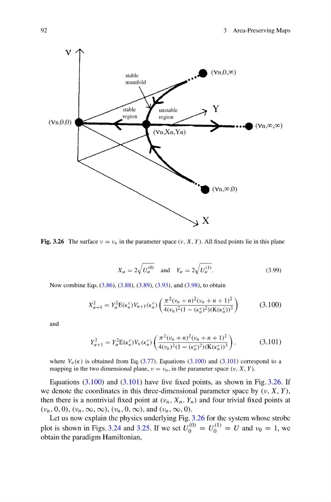
Fig. 3.26 The surface ν = ν n in the parameter space (ν, X, Y ). All fixed points lie in this plane
X α = 2
U
(0)
α
and Y α = 2
U
(1)
α .
(3.99)
Now combine Eqs. (3.86), (3.88), (3.89), (3.93), and (3.98), to obtain
X
2
α+1 = Y
2
α E(κ
c
n )V n+1 (κ
c
n )
π 2 (ν n + n) 2 (ν n + n + 1) 2
4(ν n ) 2 (1 − (κ c
n ) 2 )(K(κ c
n )) 3
(3.100)
and
Y
2
α+1 = Y
2
α E(κ
c
n )V n (κ
c
n )
π 2 (ν n + n) 2 (ν n + n + 1) 2
4(ν n ) 2 (1 − (κ c
n ) 2 )(K(κ c
n )) 3
,
(3.101)
where V n (κ) is obtained from Eq. (3.77). Equations (3.100) and (3.101) correspond to a
mapping in the two dimensional plane, ν = ν n , in the parameter space (ν, X, Y ).
Equations (3.100) and (3.101) have five fixed points, as shown in Fig. 3.26. If
we denote the coordinates in this three-dimensional parameter space by (ν, X, Y ),
then there is a nontrivial fixed point at (ν n , X n , Y n ) and four trivial fixed points at
(ν n , 0, 0), (ν n , ∞, ∞), (ν n , 0, ∞), and (ν n , ∞, 0).
Let us now explain the physics underlying Fig. 3.26 for the system whose strobe
plot is shown in Figs. 3.24 and 3.25. If we set U
(0)
0 = U
(1)
0 = U and ν 0 = 1, we
obtain the paradigm Hamiltonian,
3 Area-Preserving Maps
Fig. 3.26 The surface ν = ν n in the parameter space (ν, X, Y ). All fixed points lie in this plane
X α = 2
U
(0)
α
and Y α = 2
U
(1)
α .
(3.99)
Now combine Eqs. (3.86), (3.88), (3.89), (3.93), and (3.98), to obtain
X
2
α+1 = Y
2
α E(κ
c
n )V n+1 (κ
c
n )
π 2 (ν n + n) 2 (ν n + n + 1) 2
4(ν n ) 2 (1 − (κ c
n ) 2 )(K(κ c
n )) 3
(3.100)
and
Y
2
α+1 = Y
2
α E(κ
c
n )V n (κ
c
n )
π 2 (ν n + n) 2 (ν n + n + 1) 2
4(ν n ) 2 (1 − (κ c
n ) 2 )(K(κ c
n )) 3
,
(3.101)
where V n (κ) is obtained from Eq. (3.77). Equations (3.100) and (3.101) correspond to a
mapping in the two dimensional plane, ν = ν n , in the parameter space (ν, X, Y ).
Equations (3.100) and (3.101) have five fixed points, as shown in Fig. 3.26. If
we denote the coordinates in this three-dimensional parameter space by (ν, X, Y ),
then there is a nontrivial fixed point at (ν n , X n , Y n ) and four trivial fixed points at
(ν n , 0, 0), (ν n , ∞, ∞), (ν n , 0, ∞), and (ν n , ∞, 0).
Let us now explain the physics underlying Fig. 3.26 for the system whose strobe
plot is shown in Figs. 3.24 and 3.25. If we set U
(0)
0 = U
(1)
0 = U and ν 0 = 1, we
obtain the paradigm Hamiltonian,