

88
3 Area-Preserving Maps
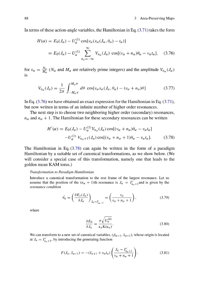
In terms of these action-angle variables, the Hamiltonian in Eq. (3.71) takes the form
H (α) = E 0 (J α ) − U
(1)
α cos[ν α (x α (J α , θ α ) − t α )]
= E 0 (J α ) − U
(1)
α
∞
n α =−∞
V n α (J α ) cos[(ν α + n α )θ α − ν α t α ], (3.76)
for ν α =
N α
M α
(N α and M α are relatively prime integers) and the amplitude V n α (J α )
is
V n α (J α ) =
1
2π
M α π
−M α π
dθ cos[ν α x α (J α , θ α ) − (ν α + n α )θ ]
(3.77)
In Eq. (3.76) we have obtained an exact expression for the Hamiltonian in Eq. (3.71),
but now written in terms of an infinite number of higher order resonances.
The next step is to choose two neighboring higher order (secondary) resonances,
n α and n α + 1. The Hamiltonian for these secondary resonances can be written
H
(α) = E 0 (J α ) − U
(1)
α V n α (J α ) cos[(ν α + n α )θ α − ν α t α ]
−U
(1)
α V n α +1 (J α ) cos[(ν α + n α + 1)θ α − ν α t α ].
(3.78)
The Hamiltonian in Eq. (3.78) can again be written in the form of a paradigm
Hamiltonian by a suitable set of canonical transformations, as we show below. (We
will consider a special case of this transformation, namely one that leads to the
golden mean KAM torus.)
Transformation to Paradigm Hamiltonian
Introduce a canonical transformation to the rest frame of the largest resonance. Let us
assume that the position of the (n α + 1)th resonance is J α = I c
nα +1 and is given by the
resonance condition
˙
θ α =
∂E o (J α )
∂J α
Jα =I c
nα +1
=
ν α
ν α + n α + 1
,
(3.79)
where
∂E 0
∂J α
=
π
U
(0)
α
κ α K(κ α )
.
(3.80)
We can transform to a new set of canonical variables, ( ¯
p α+1 , ¯
x α+1 ), whose origin is located
at J α = I c
nα +1 , by introducing the generating function
F (J α , ¯
x α+1 ) = −( ¯
x α+1 + ν α t α )
J α − I c
nα +1
ν α + n α + 1
.
(3.81)
3 Area-Preserving Maps
In terms of these action-angle variables, the Hamiltonian in Eq. (3.71) takes the form
H (α) = E 0 (J α ) − U
(1)
α cos[ν α (x α (J α , θ α ) − t α )]
= E 0 (J α ) − U
(1)
α
∞
n α =−∞
V n α (J α ) cos[(ν α + n α )θ α − ν α t α ], (3.76)
for ν α =
N α
M α
(N α and M α are relatively prime integers) and the amplitude V n α (J α )
is
V n α (J α ) =
1
2π
M α π
−M α π
dθ cos[ν α x α (J α , θ α ) − (ν α + n α )θ ]
(3.77)
In Eq. (3.76) we have obtained an exact expression for the Hamiltonian in Eq. (3.71),
but now written in terms of an infinite number of higher order resonances.
The next step is to choose two neighboring higher order (secondary) resonances,
n α and n α + 1. The Hamiltonian for these secondary resonances can be written
H
(α) = E 0 (J α ) − U
(1)
α V n α (J α ) cos[(ν α + n α )θ α − ν α t α ]
−U
(1)
α V n α +1 (J α ) cos[(ν α + n α + 1)θ α − ν α t α ].
(3.78)
The Hamiltonian in Eq. (3.78) can again be written in the form of a paradigm
Hamiltonian by a suitable set of canonical transformations, as we show below. (We
will consider a special case of this transformation, namely one that leads to the
golden mean KAM torus.)
Transformation to Paradigm Hamiltonian
Introduce a canonical transformation to the rest frame of the largest resonance. Let us
assume that the position of the (n α + 1)th resonance is J α = I c
nα +1 and is given by the
resonance condition
˙
θ α =
∂E o (J α )
∂J α
Jα =I c
nα +1
=
ν α
ν α + n α + 1
,
(3.79)
where
∂E 0
∂J α
=
π
U
(0)
α
κ α K(κ α )
.
(3.80)
We can transform to a new set of canonical variables, ( ¯
p α+1 , ¯
x α+1 ), whose origin is located
at J α = I c
nα +1 , by introducing the generating function
F (J α , ¯
x α+1 ) = −( ¯
x α+1 + ν α t α )
J α − I c
nα +1
ν α + n α + 1
.
(3.81)