

3.8 Renormalization Map
89
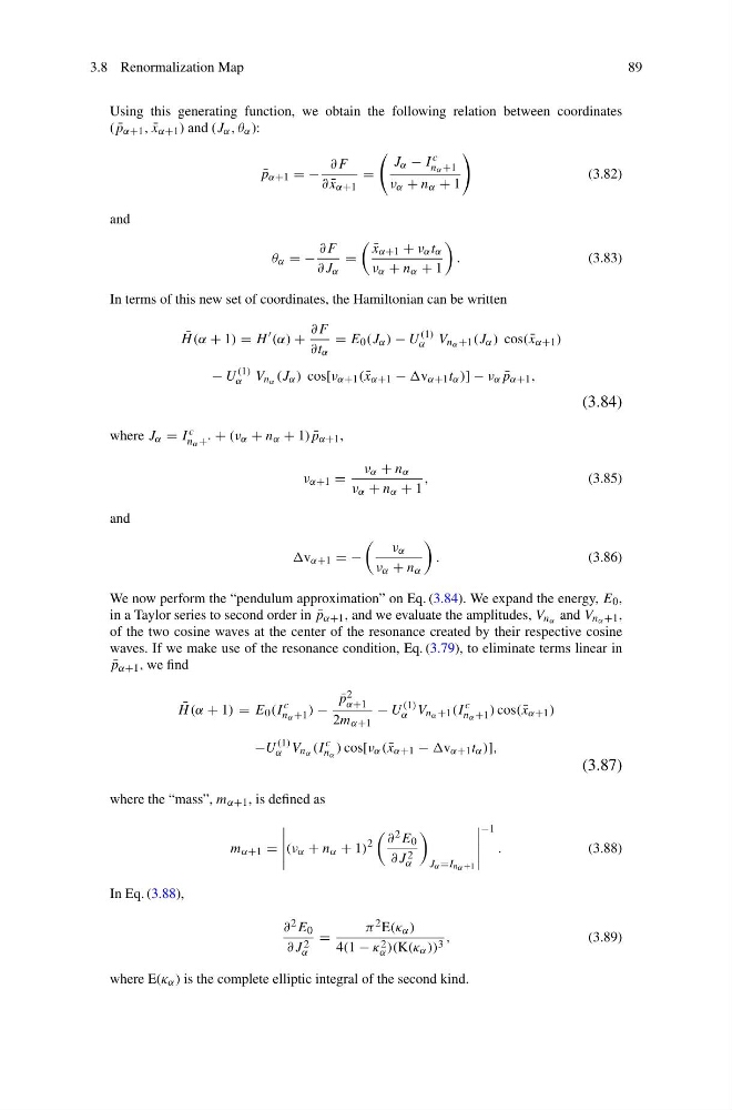
Using this generating function, we obtain the following relation between coordinates
( ¯
p α+1 , ¯
x α+1 ) and (J α , θ α ):
¯
p α+1 = −
∂F
∂ ¯
x α+1
=
J α − I c
nα +1
ν α + n α + 1
(3.82)
and
θ α = −
∂F
∂J α
=
¯
x α+1 + ν α t α
ν α + n α + 1
.
(3.83)
In terms of this new set of coordinates, the Hamiltonian can be written
¯
H (α + 1) = H
(α) +
∂F
∂t α
= E 0 (J α ) − U
(1)
α V nα +1 (J α ) cos( ¯
x α+1 )
− U
(1)
α V nα (J α ) cos[ν α+1 ( ¯
x α+1 − v α+1 t α )] − ν α ¯
p α+1 ,
(3.84)
where J α = I c
nα +‘ + (ν α + n α + 1) ¯
p α+1 ,
ν α+1 =
ν α + n α
ν α + n α + 1
,
(3.85)
and
v α+1 = −
ν α
ν α + n α
.
(3.86)
We now perform the “pendulum approximation” on Eq. (3.84). We expand the energy, E 0 ,
in a Taylor series to second order in ¯
p α+1 , and we evaluate the amplitudes, V nα and V nα +1 ,
of the two cosine waves at the center of the resonance created by their respective cosine
waves. If we make use of the resonance condition, Eq. (3.79), to eliminate terms linear in
¯
p α+1 , we find
¯
H (α + 1) = E 0 (I
c
nα +1 ) −
¯
p 2
α+1
2m α+1
− U
(1)
α V nα +1 (I
c
nα +1 ) cos( ¯
x α+1 )
−U
(1)
α V nα (I
c
nα ) cos[ν α ( ¯
x α+1 − v α+1 t α )],
(3.87)
where the “mass”, m α+1 , is defined as
m α+1 =
(ν α + n α + 1)
2
∂ 2 E 0
∂J 2
α
Jα =I nα +1
−1
.
(3.88)
In Eq. (3.88),
∂ 2 E 0
∂J 2
α
=
π 2 E(κ α )
4(1 − κ 2
α )(K(κ α )) 3 ,
(3.89)
where E(κ α ) is the complete elliptic integral of the second kind.
89
Using this generating function, we obtain the following relation between coordinates
( ¯
p α+1 , ¯
x α+1 ) and (J α , θ α ):
¯
p α+1 = −
∂F
∂ ¯
x α+1
=
J α − I c
nα +1
ν α + n α + 1
(3.82)
and
θ α = −
∂F
∂J α
=
¯
x α+1 + ν α t α
ν α + n α + 1
.
(3.83)
In terms of this new set of coordinates, the Hamiltonian can be written
¯
H (α + 1) = H
(α) +
∂F
∂t α
= E 0 (J α ) − U
(1)
α V nα +1 (J α ) cos( ¯
x α+1 )
− U
(1)
α V nα (J α ) cos[ν α+1 ( ¯
x α+1 − v α+1 t α )] − ν α ¯
p α+1 ,
(3.84)
where J α = I c
nα +‘ + (ν α + n α + 1) ¯
p α+1 ,
ν α+1 =
ν α + n α
ν α + n α + 1
,
(3.85)
and
v α+1 = −
ν α
ν α + n α
.
(3.86)
We now perform the “pendulum approximation” on Eq. (3.84). We expand the energy, E 0 ,
in a Taylor series to second order in ¯
p α+1 , and we evaluate the amplitudes, V nα and V nα +1 ,
of the two cosine waves at the center of the resonance created by their respective cosine
waves. If we make use of the resonance condition, Eq. (3.79), to eliminate terms linear in
¯
p α+1 , we find
¯
H (α + 1) = E 0 (I
c
nα +1 ) −
¯
p 2
α+1
2m α+1
− U
(1)
α V nα +1 (I
c
nα +1 ) cos( ¯
x α+1 )
−U
(1)
α V nα (I
c
nα ) cos[ν α ( ¯
x α+1 − v α+1 t α )],
(3.87)
where the “mass”, m α+1 , is defined as
m α+1 =
(ν α + n α + 1)
2
∂ 2 E 0
∂J 2
α
Jα =I nα +1
−1
.
(3.88)
In Eq. (3.88),
∂ 2 E 0
∂J 2
α
=
π 2 E(κ α )
4(1 − κ 2
α )(K(κ α )) 3 ,
(3.89)
where E(κ α ) is the complete elliptic integral of the second kind.