

3.8 Renormalization Map
87
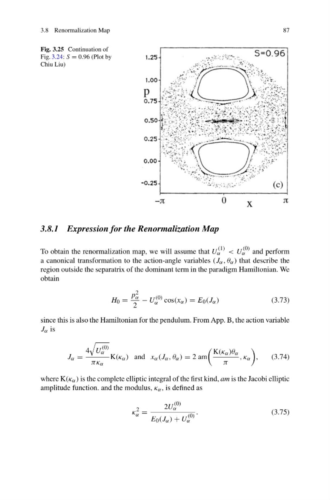
Fig. 3.25 Continuation of
Fig. 3.24: S = 0.96 (Plot by
Chiu Liu)
3.8.1 Expression for the Renormalization Map
To obtain the renormalization map, we will assume that U
(1)
α < U
(0)
α and perform
a canonical transformation to the action-angle variables (J α , θ α ) that describe the
region outside the separatrix of the dominant term in the paradigm Hamiltonian. We
obtain
H 0 =
p 2
α
2
− U
(0)
α cos(x α ) = E 0 (J α )
(3.73)
since this is also the Hamiltonian for the pendulum. From App. B, the action variable
J α is
J α =
4
U
(0)
α
πκ α
K(κ α ) and x α (J α , θ α ) = 2 am
K(κ α )θ α
π
, κ α
,
(3.74)
where K(κ α ) is the complete elliptic integral of the first kind, am is the Jacobi elliptic
amplitude function. and the modulus, κ α , is defined as
κ
2
α =
2U
(0)
α
E 0 (J α ) + U
(0)
α
.
(3.75)
87
Fig. 3.25 Continuation of
Fig. 3.24: S = 0.96 (Plot by
Chiu Liu)
3.8.1 Expression for the Renormalization Map
To obtain the renormalization map, we will assume that U
(1)
α < U
(0)
α and perform
a canonical transformation to the action-angle variables (J α , θ α ) that describe the
region outside the separatrix of the dominant term in the paradigm Hamiltonian. We
obtain
H 0 =
p 2
α
2
− U
(0)
α cos(x α ) = E 0 (J α )
(3.73)
since this is also the Hamiltonian for the pendulum. From App. B, the action variable
J α is
J α =
4
U
(0)
α
πκ α
K(κ α ) and x α (J α , θ α ) = 2 am
K(κ α )θ α
π
, κ α
,
(3.74)
where K(κ α ) is the complete elliptic integral of the first kind, am is the Jacobi elliptic
amplitude function. and the modulus, κ α , is defined as
κ
2
α =
2U
(0)
α
E 0 (J α ) + U
(0)
α
.
(3.75)