

530
A. Doikou et al.
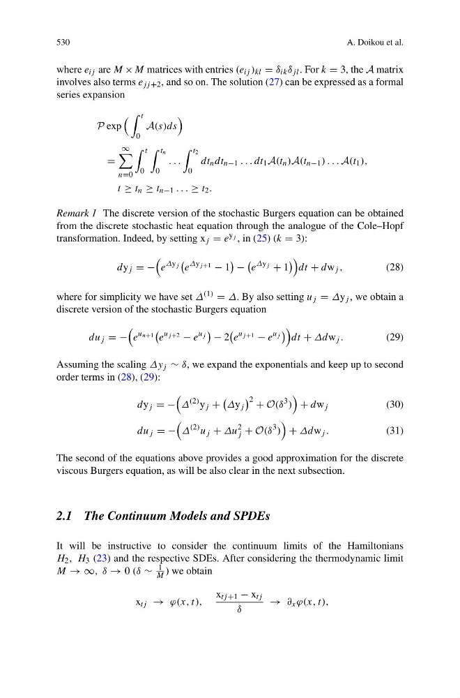
where e ij are M × M matrices with entries (e ij ) kl = δ ik δ jl . For k = 3, the A matrix
involves also terms e jj +2 , and so on. The solution (27) can be expressed as a formal
series expansion
P exp
t
0
A(s)ds
=
∞
n=0
t
0
t n
0
. . .
t 2
0
dt n dt n−1 . . . dt 1 A(t n )A(t n−1 ) . . . A(t 1 ),
t ≥ t n ≥ t n−1 . . . ≥ t 2 .
Remark 1 The discrete version of the stochastic Burgers equation can be obtained
from the discrete stochastic heat equation through the analogue of the Cole–Hopf
transformation. Indeed, by setting x j = e y j , in (25) (k = 3):
dy j = −
e
Δy j
e
Δy j +1 − 1
−
e
Δy j + 1
dt + dw j ,
(28)
where for simplicity we have set Δ (1) = Δ. By also setting u j = Δy j , we obtain a
discrete version of the stochastic Burgers equation
du j = −
e
u n+1
e
u j +2 − e
u j
− 2
e
u j +1 − e
u j
dt + Δdw j .
(29)
Assuming the scaling Δy j ∼ δ, we expand the exponentials and keep up to second
order terms in (28), (29):
dy j = −
Δ
(2) y j +
Δy j
2 + O(δ
3 )
+ dw j
(30)
du j = −
Δ
(2) u j + Δu
2
j + O(δ
3 )
+ Δdw j .
(31)
The second of the equations above provides a good approximation for the discrete
viscous Burgers equation, as will be also clear in the next subsection.
2.1 The Continuum Models and SPDEs
It will be instructive to consider the continuum limits of the Hamiltonians
H 2 , H 3 (23) and the respective SDEs. After considering the thermodynamic limit
M → ∞, δ → 0 (δ ∼
1
M ) we obtain
x tj → ϕ(x, t),
x tj +1 − x tj
δ
→ ∂ x ϕ(x, t),
A. Doikou et al.
where e ij are M × M matrices with entries (e ij ) kl = δ ik δ jl . For k = 3, the A matrix
involves also terms e jj +2 , and so on. The solution (27) can be expressed as a formal
series expansion
P exp
t
0
A(s)ds
=
∞
n=0
t
0
t n
0
. . .
t 2
0
dt n dt n−1 . . . dt 1 A(t n )A(t n−1 ) . . . A(t 1 ),
t ≥ t n ≥ t n−1 . . . ≥ t 2 .
Remark 1 The discrete version of the stochastic Burgers equation can be obtained
from the discrete stochastic heat equation through the analogue of the Cole–Hopf
transformation. Indeed, by setting x j = e y j , in (25) (k = 3):
dy j = −
e
Δy j
e
Δy j +1 − 1
−
e
Δy j + 1
dt + dw j ,
(28)
where for simplicity we have set Δ (1) = Δ. By also setting u j = Δy j , we obtain a
discrete version of the stochastic Burgers equation
du j = −
e
u n+1
e
u j +2 − e
u j
− 2
e
u j +1 − e
u j
dt + Δdw j .
(29)
Assuming the scaling Δy j ∼ δ, we expand the exponentials and keep up to second
order terms in (28), (29):
dy j = −
Δ
(2) y j +
Δy j
2 + O(δ
3 )
+ dw j
(30)
du j = −
Δ
(2) u j + Δu
2
j + O(δ
3 )
+ Δdw j .
(31)
The second of the equations above provides a good approximation for the discrete
viscous Burgers equation, as will be also clear in the next subsection.
2.1 The Continuum Models and SPDEs
It will be instructive to consider the continuum limits of the Hamiltonians
H 2 , H 3 (23) and the respective SDEs. After considering the thermodynamic limit
M → ∞, δ → 0 (δ ∼
1
M ) we obtain
x tj → ϕ(x, t),
x tj +1 − x tj
δ
→ ∂ x ϕ(x, t),