

Time Evolution in Quantum Systems and Stochastics
529
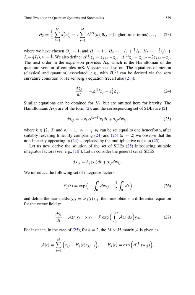
H 3 =
1
2
M
j =1
x
2
j ∂
2
x j
− ν
M
j =1
Δ
(2) (x j )∂ x j + (higher order terms) . . . ,
(23)
where we have chosen Θ j = 1, and H 1 = I 1 , H 2 = −I 2 +
1
2 I 1 , H 3 = −
1
3
I 3 +
I 2 −
1
2 I 1 ), ν =
1
3 . We also define: Δ (1) z j = z j +1 −z j , Δ (2) z j = z j +2 −2z j +1 +z j .
The next order in the expansion provides H 4 , which is the Hamiltonian of the
quantum version of complex mKdV system and so on. The equations of motion
(classical and quantum) associated, e.g., with H (2) can be derived via the zero
curvature condition or Heisenberg’s equation (recall also (21)):
dz j
dt
= −Δ
(1) z j + z
2
j Z j .
(24)
Similar equations can be obtained for H 3 , but are omitted here for brevity. The
Hamiltonians H 2,3 are of the form (2), and the corresponding set of SDEs are [2]
dx tj = −ν k Δ
(k−1) x t dt + x tj dw tj ,
(25)
where k ∈ {2, 3} and ν 2 = 1, ν 3 =
1
3 . ν k can be set equal to one henceforth, after
suitably rescaling time. By comparing (24) and (25) (k = 2) we observe that the
non-linearity appearing in (24) is replaced by the multiplicative noise in (25).
Let us now derive the solution of the set of SDEs (25) introducing suitable
integrator factors (see, e.g., [10]). Let us consider the general set of SDES
dx tj = b j (x t )dt + x tj dw tj .
We introduce the following set of integrator factors:
F j (t) = exp
−
t
0
dw sj +
1
2
t
0
ds
(26)
and define the new fields: y tj = F j (t)x tj , then one obtains a differential equation
for the vector field y:
dy t
dt
= A(t)y t ⇒ y t = P exp
t
0
A(s)ds
y 0 .
(27)
For instance, in the case of (25), for k = 2, the M × M matrix A is given as
A(t) =
M
j =1
e jj − B j (t)e jj +1
,
B j (t) = exp
Δ
(1) (w tj )
,
529
H 3 =
1
2
M
j =1
x
2
j ∂
2
x j
− ν
M
j =1
Δ
(2) (x j )∂ x j + (higher order terms) . . . ,
(23)
where we have chosen Θ j = 1, and H 1 = I 1 , H 2 = −I 2 +
1
2 I 1 , H 3 = −
1
3
I 3 +
I 2 −
1
2 I 1 ), ν =
1
3 . We also define: Δ (1) z j = z j +1 −z j , Δ (2) z j = z j +2 −2z j +1 +z j .
The next order in the expansion provides H 4 , which is the Hamiltonian of the
quantum version of complex mKdV system and so on. The equations of motion
(classical and quantum) associated, e.g., with H (2) can be derived via the zero
curvature condition or Heisenberg’s equation (recall also (21)):
dz j
dt
= −Δ
(1) z j + z
2
j Z j .
(24)
Similar equations can be obtained for H 3 , but are omitted here for brevity. The
Hamiltonians H 2,3 are of the form (2), and the corresponding set of SDEs are [2]
dx tj = −ν k Δ
(k−1) x t dt + x tj dw tj ,
(25)
where k ∈ {2, 3} and ν 2 = 1, ν 3 =
1
3 . ν k can be set equal to one henceforth, after
suitably rescaling time. By comparing (24) and (25) (k = 2) we observe that the
non-linearity appearing in (24) is replaced by the multiplicative noise in (25).
Let us now derive the solution of the set of SDEs (25) introducing suitable
integrator factors (see, e.g., [10]). Let us consider the general set of SDES
dx tj = b j (x t )dt + x tj dw tj .
We introduce the following set of integrator factors:
F j (t) = exp
−
t
0
dw sj +
1
2
t
0
ds
(26)
and define the new fields: y tj = F j (t)x tj , then one obtains a differential equation
for the vector field y:
dy t
dt
= A(t)y t ⇒ y t = P exp
t
0
A(s)ds
y 0 .
(27)
For instance, in the case of (25), for k = 2, the M × M matrix A is given as
A(t) =
M
j =1
e jj − B j (t)e jj +1
,
B j (t) = exp
Δ
(1) (w tj )
,