

528
A. Doikou et al.
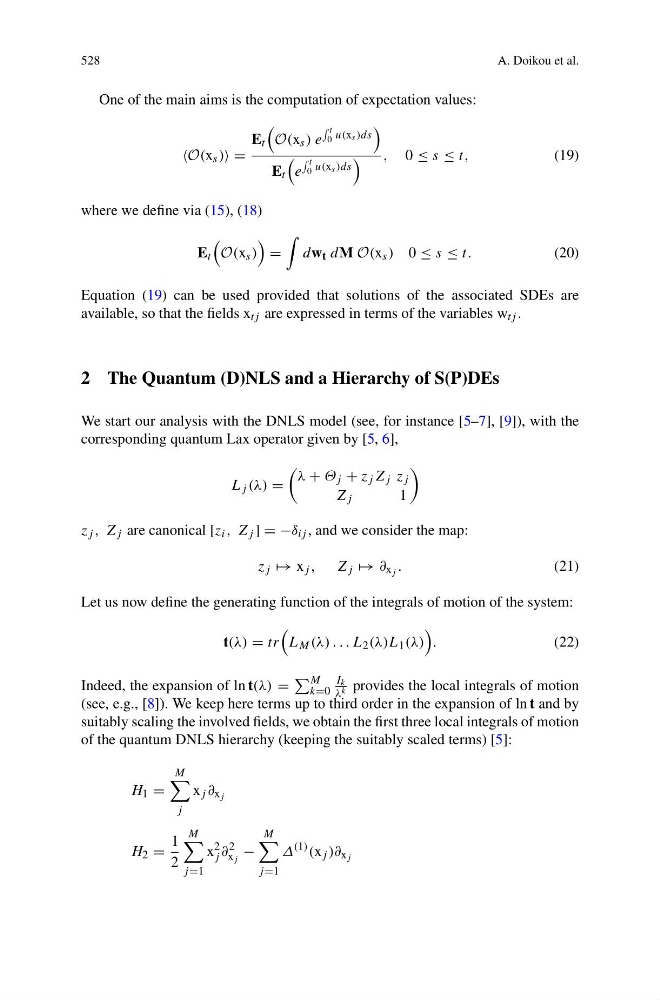
One of the main aims is the computation of expectation values:
s ) =
E t
O(x s ) e
t
0 u(x s )ds
E t
e
t
0 u(x s )ds
, 0 ≤ s ≤ t,
(19)
where we define via (15), (18)
E t
O(x s )
=
dw t dM O(x s ) 0 ≤ s ≤ t.
(20)
Equation (19) can be used provided that solutions of the associated SDEs are
available, so that the fields x tj are expressed in terms of the variables w tj .
2 The Quantum (D)NLS and a Hierarchy of S(P)DEs
We start our analysis with the DNLS model (see, for instance [5–7], [9]), with the
corresponding quantum Lax operator given by [5, 6],
L j (λ) =
λ + Θ j + z j Z j z j
Z j
1
z j , Z j are canonical [z i , Z j ] = −δ ij , and we consider the map:
z j → x j , Z j → ∂ x j .
(21)
Let us now define the generating function of the integrals of motion of the system:
t(λ) = tr
L M (λ) . . . L 2 (λ)L 1 (λ)
.
(22)
Indeed, the expansion of ln t(λ) =
M
k=0
I k
λ k provides the local integrals of motion
(see, e.g., [8]). We keep here terms up to third order in the expansion of ln t and by
suitably scaling the involved fields, we obtain the first three local integrals of motion
of the quantum DNLS hierarchy (keeping the suitably scaled terms) [5]:
H 1 =
M
j
x j ∂ x j
H 2 =
1
2
M
j =1
x
2
j ∂
2
x j
−
M
j =1
Δ
(1) (x j )∂ x j
A. Doikou et al.
One of the main aims is the computation of expectation values:
s ) =
E t
O(x s ) e
t
0 u(x s )ds
E t
e
t
0 u(x s )ds
, 0 ≤ s ≤ t,
(19)
where we define via (15), (18)
E t
O(x s )
=
dw t dM O(x s ) 0 ≤ s ≤ t.
(20)
Equation (19) can be used provided that solutions of the associated SDEs are
available, so that the fields x tj are expressed in terms of the variables w tj .
2 The Quantum (D)NLS and a Hierarchy of S(P)DEs
We start our analysis with the DNLS model (see, for instance [5–7], [9]), with the
corresponding quantum Lax operator given by [5, 6],
L j (λ) =
λ + Θ j + z j Z j z j
Z j
1
z j , Z j are canonical [z i , Z j ] = −δ ij , and we consider the map:
z j → x j , Z j → ∂ x j .
(21)
Let us now define the generating function of the integrals of motion of the system:
t(λ) = tr
L M (λ) . . . L 2 (λ)L 1 (λ)
.
(22)
Indeed, the expansion of ln t(λ) =
M
k=0
I k
λ k provides the local integrals of motion
(see, e.g., [8]). We keep here terms up to third order in the expansion of ln t and by
suitably scaling the involved fields, we obtain the first three local integrals of motion
of the quantum DNLS hierarchy (keeping the suitably scaled terms) [5]:
H 1 =
M
j
x j ∂ x j
H 2 =
1
2
M
j =1
x
2
j ∂
2
x j
−
M
j =1
Δ
(1) (x j )∂ x j