

Time Evolution in Quantum Systems and Stochastics
527
dM = lim
δ→0
lim
N →∞
1
(2πδ)
NM
2
exp
−
1
2δ
N
n=1
Δw
T
n Δw n
N
n=2
M
j =1
dw jn .
(16)
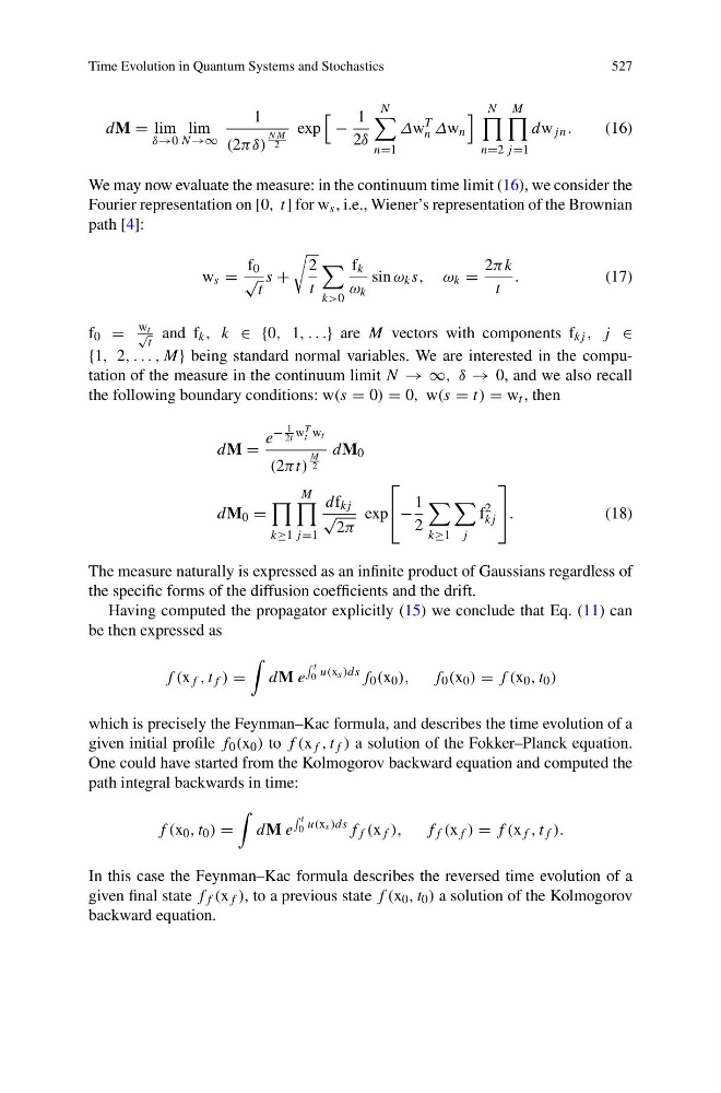
We may now evaluate the measure: in the continuum time limit (16), we consider the
Fourier representation on [0, t] for w s , i.e., Wiener’s representation of the Brownian
path [4]:
w s =
f 0
√
t
s +
2
t
k>0
f k
ω k
sin ω k s, ω k =
2πk
t
.
(17)
f 0 =
w t
√
t
and f k , k ∈ {0, 1, . . .} are M vectors with components f kj , j ∈
{1, 2, . . . , M} being standard normal variables. We are interested in the computation of the measure in the continuum limit N → ∞, δ → 0, and we also recall
the following boundary conditions: w(s = 0) = 0, w(s = t) = w t , then
dM =
e
−
1
2t w T
t w t
(2πt)
M
2
dM 0
dM 0 =
k≥1
M
j =1
df kj
√
2π
exp
⎡
⎣ −
1
2
k≥1
j
f
2
kj
⎤
⎦ .
(18)
The measure naturally is expressed as an infinite product of Gaussians regardless of
the specific forms of the diffusion coefficients and the drift.
Having computed the propagator explicitly (15) we conclude that Eq. (11) can
be then expressed as
f (x f , t f ) =
dM e
t
0 u(x s )ds f 0 (x 0 ), f 0 (x 0 ) = f (x 0 , t 0 )
which is precisely the Feynman–Kac formula, and describes the time evolution of a
given initial profile f 0 (x 0 ) to f (x f , t f ) a solution of the Fokker–Planck equation.
One could have started from the Kolmogorov backward equation and computed the
path integral backwards in time:
f (x 0 , t 0 ) =
dM e
t
0 u(x s )ds f f (x f ), f f (x f ) = f (x f , t f ).
In this case the Feynman–Kac formula describes the reversed time evolution of a
given final state f f (x f ), to a previous state f (x 0 , t 0 ) a solution of the Kolmogorov
backward equation.
527
dM = lim
δ→0
lim
N →∞
1
(2πδ)
NM
2
exp
−
1
2δ
N
n=1
Δw
T
n Δw n
N
n=2
M
j =1
dw jn .
(16)
We may now evaluate the measure: in the continuum time limit (16), we consider the
Fourier representation on [0, t] for w s , i.e., Wiener’s representation of the Brownian
path [4]:
w s =
f 0
√
t
s +
2
t
k>0
f k
ω k
sin ω k s, ω k =
2πk
t
.
(17)
f 0 =
w t
√
t
and f k , k ∈ {0, 1, . . .} are M vectors with components f kj , j ∈
{1, 2, . . . , M} being standard normal variables. We are interested in the computation of the measure in the continuum limit N → ∞, δ → 0, and we also recall
the following boundary conditions: w(s = 0) = 0, w(s = t) = w t , then
dM =
e
−
1
2t w T
t w t
(2πt)
M
2
dM 0
dM 0 =
k≥1
M
j =1
df kj
√
2π
exp
⎡
⎣ −
1
2
k≥1
j
f
2
kj
⎤
⎦ .
(18)
The measure naturally is expressed as an infinite product of Gaussians regardless of
the specific forms of the diffusion coefficients and the drift.
Having computed the propagator explicitly (15) we conclude that Eq. (11) can
be then expressed as
f (x f , t f ) =
dM e
t
0 u(x s )ds f 0 (x 0 ), f 0 (x 0 ) = f (x 0 , t 0 )
which is precisely the Feynman–Kac formula, and describes the time evolution of a
given initial profile f 0 (x 0 ) to f (x f , t f ) a solution of the Fokker–Planck equation.
One could have started from the Kolmogorov backward equation and computed the
path integral backwards in time:
f (x 0 , t 0 ) =
dM e
t
0 u(x s )ds f f (x f ), f f (x f ) = f (x f , t f ).
In this case the Feynman–Kac formula describes the reversed time evolution of a
given final state f f (x f ), to a previous state f (x 0 , t 0 ) a solution of the Kolmogorov
backward equation.