

526
A. Doikou et al.
1.2 The Path Integral: Feynman–Kac Formula
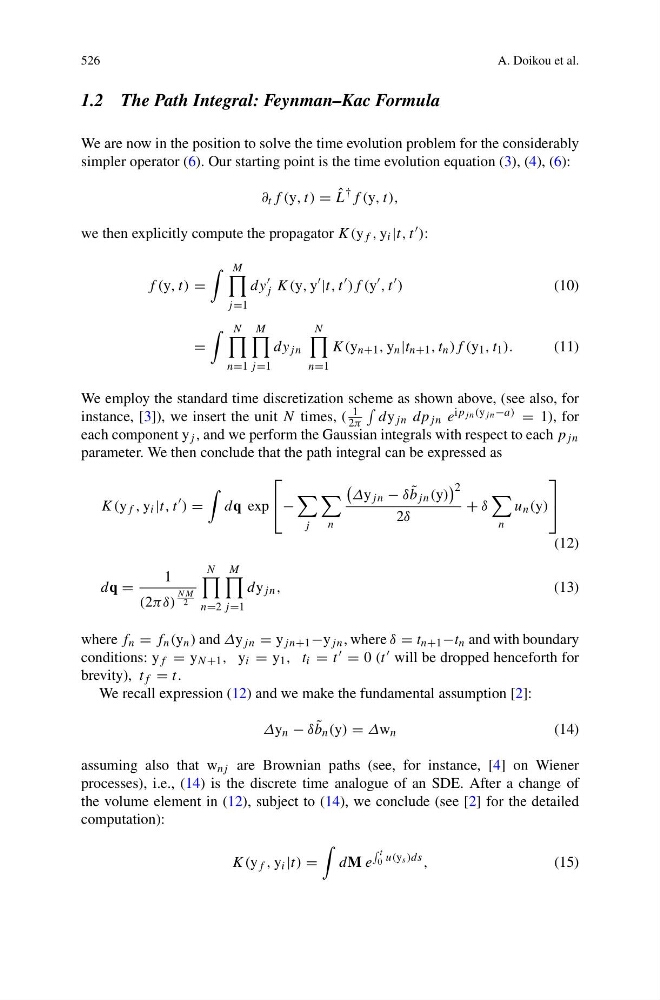
We are now in the position to solve the time evolution problem for the considerably
simpler operator (6). Our starting point is the time evolution equation (3), (4), (6):
∂ t f (y, t) = ˆ
L
† f (y, t),
we then explicitly compute the propagator K(y f , y i |t, t ):
f (y, t) =
M
j =1
dy
j K(y, y
|t, t
)f (y
, t
)
(10)
=
N
n=1
M
j =1
dy jn
N
n=1
K(y n+1 , y n |t n+1 , t n )f (y 1 , t 1 ).
(11)
We employ the standard time discretization scheme as shown above, (see also, for
instance, [3]), we insert the unit N times, (
1
2π
dy jn dp jn e ip jn (y jn −a) = 1), for
each component y j , and we perform the Gaussian integrals with respect to each p jn
parameter. We then conclude that the path integral can be expressed as
K(y f , y i |t, t
) =
dq exp
⎡
⎣ −
j
n
Δy jn − δ ˜
b jn (y)
2
2δ
+ δ
n
u n (y)
⎤
⎦
(12)
dq =
1
(2πδ)
NM
2
N
n=2
M
j =1
dy jn ,
(13)
where f n = f n (y n ) and Δy jn = y jn+1 −y jn , where δ = t n+1 −t n and with boundary
conditions: y f = y N +1 , y i = y 1 , t i = t = 0 (t will be dropped henceforth for
brevity), t f = t.
We recall expression (12) and we make the fundamental assumption [2]:
Δy n − δ ˜
b n (y) = Δw n
(14)
assuming also that w nj are Brownian paths (see, for instance, [4] on Wiener
processes), i.e., (14) is the discrete time analogue of an SDE. After a change of
the volume element in (12), subject to (14), we conclude (see [2] for the detailed
computation):
K(y f , y i |t) =
dM e
t
0 u(y s )ds ,
(15)
A. Doikou et al.
1.2 The Path Integral: Feynman–Kac Formula
We are now in the position to solve the time evolution problem for the considerably
simpler operator (6). Our starting point is the time evolution equation (3), (4), (6):
∂ t f (y, t) = ˆ
L
† f (y, t),
we then explicitly compute the propagator K(y f , y i |t, t ):
f (y, t) =
M
j =1
dy
j K(y, y
|t, t
)f (y
, t
)
(10)
=
N
n=1
M
j =1
dy jn
N
n=1
K(y n+1 , y n |t n+1 , t n )f (y 1 , t 1 ).
(11)
We employ the standard time discretization scheme as shown above, (see also, for
instance, [3]), we insert the unit N times, (
1
2π
dy jn dp jn e ip jn (y jn −a) = 1), for
each component y j , and we perform the Gaussian integrals with respect to each p jn
parameter. We then conclude that the path integral can be expressed as
K(y f , y i |t, t
) =
dq exp
⎡
⎣ −
j
n
Δy jn − δ ˜
b jn (y)
2
2δ
+ δ
n
u n (y)
⎤
⎦
(12)
dq =
1
(2πδ)
NM
2
N
n=2
M
j =1
dy jn ,
(13)
where f n = f n (y n ) and Δy jn = y jn+1 −y jn , where δ = t n+1 −t n and with boundary
conditions: y f = y N +1 , y i = y 1 , t i = t = 0 (t will be dropped henceforth for
brevity), t f = t.
We recall expression (12) and we make the fundamental assumption [2]:
Δy n − δ ˜
b n (y) = Δw n
(14)
assuming also that w nj are Brownian paths (see, for instance, [4] on Wiener
processes), i.e., (14) is the discrete time analogue of an SDE. After a change of
the volume element in (12), subject to (14), we conclude (see [2] for the detailed
computation):
K(y f , y i |t) =
dM e
t
0 u(y s )ds ,
(15)