

Time Evolution in Quantum Systems and Stochastics
525
1 Time Evolution and the Feynman–Kac Formula
Before we compute the solution of the time evolution problem via the path integral
formulation we shall implement the quantum canonical transform that turns the
dynamical diffusion matrix in (2) into identity at the level of the PDEs. This result
will be then used for the explicit computation of the general path integral, and the
derivation of the Feynman–Kac formula [2].
1.1 The Quantum Canonical Transformation
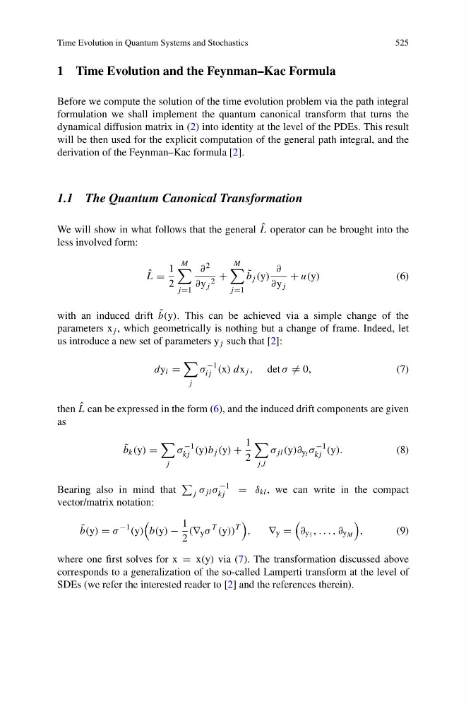
We will show in what follows that the general ˆ
L operator can be brought into the
less involved form:
ˆ
L =
1
2
M
j =1
∂ 2
∂y j
2
+
M
j =1
˜
b j (y)
∂
∂y j
+ u(y)
(6)
with an induced drift ˜
b(y). This can be achieved via a simple change of the
parameters x j , which geometrically is nothing but a change of frame. Indeed, let
us introduce a new set of parameters y j such that [2]:
dy i =
j
σ
−1
ij (x) dx j , det σ = 0,
(7)
then ˆ
L can be expressed in the form (6), and the induced drift components are given
as
˜
b k (y) =
j
σ
−1
kj (y)b j (y) +
1
2
j,l
σ jl (y)∂ y l σ
−1
kj (y).
(8)
Bearing also in mind that
j σ jl σ
−1
kj
= δ kl , we can write in the compact
vector/matrix notation:
˜
b(y) = σ
−1 (y)
b(y) −
1
2
(∇ y σ
T (y))
T
,
∇ y =
∂ y 1 , . . . , ∂ y M
,
(9)
where one first solves for x = x(y) via (7). The transformation discussed above
corresponds to a generalization of the so-called Lamperti transform at the level of
SDEs (we refer the interested reader to [2] and the references therein).
525
1 Time Evolution and the Feynman–Kac Formula
Before we compute the solution of the time evolution problem via the path integral
formulation we shall implement the quantum canonical transform that turns the
dynamical diffusion matrix in (2) into identity at the level of the PDEs. This result
will be then used for the explicit computation of the general path integral, and the
derivation of the Feynman–Kac formula [2].
1.1 The Quantum Canonical Transformation
We will show in what follows that the general ˆ
L operator can be brought into the
less involved form:
ˆ
L =
1
2
M
j =1
∂ 2
∂y j
2
+
M
j =1
˜
b j (y)
∂
∂y j
+ u(y)
(6)
with an induced drift ˜
b(y). This can be achieved via a simple change of the
parameters x j , which geometrically is nothing but a change of frame. Indeed, let
us introduce a new set of parameters y j such that [2]:
dy i =
j
σ
−1
ij (x) dx j , det σ = 0,
(7)
then ˆ
L can be expressed in the form (6), and the induced drift components are given
as
˜
b k (y) =
j
σ
−1
kj (y)b j (y) +
1
2
j,l
σ jl (y)∂ y l σ
−1
kj (y).
(8)
Bearing also in mind that
j σ jl σ
−1
kj
= δ kl , we can write in the compact
vector/matrix notation:
˜
b(y) = σ
−1 (y)
b(y) −
1
2
(∇ y σ
T (y))
T
,
∇ y =
∂ y 1 , . . . , ∂ y M
,
(9)
where one first solves for x = x(y) via (7). The transformation discussed above
corresponds to a generalization of the so-called Lamperti transform at the level of
SDEs (we refer the interested reader to [2] and the references therein).