

374
G. Barnich and M. Bonte
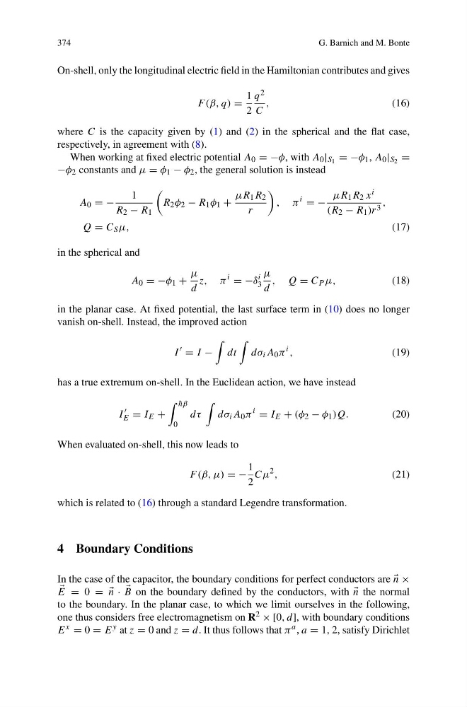
On-shell, only the longitudinal electric field in the Hamiltonian contributes and gives
F (β, q) =
1
2
q 2
C
,
(16)
where C is the capacity given by (1) and (2) in the spherical and the flat case,
respectively, in agreement with (8).
When working at fixed electric potential A 0 = −φ, with A 0 | S 1 = −φ 1 , A 0 | S 2 =
−φ 2 constants and μ = φ 1 − φ 2 , the general solution is instead
A 0 = −
1
R 2 − R 1
R 2 φ 2 − R 1 φ 1 +
μR 1 R 2
r
, π
i
= −
μR 1 R 2 x i
(R 2 − R 1 )r 3 ,
Q = C S μ,
(17)
in the spherical and
A 0 = −φ 1 +
μ
d
z, π
i
= −δ
i
3
μ
d
, Q = C P μ,
(18)
in the planar case. At fixed potential, the last surface term in (10) does no longer
vanish on-shell. Instead, the improved action
I
= I −
dt
dσ i A 0 π
i ,
(19)
has a true extremum on-shell. In the Euclidean action, we have instead
I
E = I E +
¯
hβ
0
dτ
dσ i A 0 π
i
= I E + (φ 2 − φ 1 )Q.
(20)
When evaluated on-shell, this now leads to
F (β, μ) = −
1
2
Cμ
2 ,
(21)
which is related to (16) through a standard Legendre transformation.
4 Boundary Conditions
In the case of the capacitor, the boundary conditions for perfect conductors are
n ×
E = 0 = =
n ·
B on the boundary defined by the conductors, with
n the normal
to the boundary. In the planar case, to which we limit ourselves in the following,
one thus considers free electromagnetism on R 2 × [0, d], with boundary conditions
E x = 0 = E y at z = 0 and z = d. It thus follows that π a , a = 1, 2, satisfy Dirichlet
G. Barnich and M. Bonte
On-shell, only the longitudinal electric field in the Hamiltonian contributes and gives
F (β, q) =
1
2
q 2
C
,
(16)
where C is the capacity given by (1) and (2) in the spherical and the flat case,
respectively, in agreement with (8).
When working at fixed electric potential A 0 = −φ, with A 0 | S 1 = −φ 1 , A 0 | S 2 =
−φ 2 constants and μ = φ 1 − φ 2 , the general solution is instead
A 0 = −
1
R 2 − R 1
R 2 φ 2 − R 1 φ 1 +
μR 1 R 2
r
, π
i
= −
μR 1 R 2 x i
(R 2 − R 1 )r 3 ,
Q = C S μ,
(17)
in the spherical and
A 0 = −φ 1 +
μ
d
z, π
i
= −δ
i
3
μ
d
, Q = C P μ,
(18)
in the planar case. At fixed potential, the last surface term in (10) does no longer
vanish on-shell. Instead, the improved action
I
= I −
dt
dσ i A 0 π
i ,
(19)
has a true extremum on-shell. In the Euclidean action, we have instead
I
E = I E +
¯
hβ
0
dτ
dσ i A 0 π
i
= I E + (φ 2 − φ 1 )Q.
(20)
When evaluated on-shell, this now leads to
F (β, μ) = −
1
2
Cμ
2 ,
(21)
which is related to (16) through a standard Legendre transformation.
4 Boundary Conditions
In the case of the capacitor, the boundary conditions for perfect conductors are
n ×
E = 0 = =
n ·
B on the boundary defined by the conductors, with
n the normal
to the boundary. In the planar case, to which we limit ourselves in the following,
one thus considers free electromagnetism on R 2 × [0, d], with boundary conditions
E x = 0 = E y at z = 0 and z = d. It thus follows that π a , a = 1, 2, satisfy Dirichlet