

Soft Degrees of Freedom, Gibbons–Hawking Contribution and Entropy from. . .
373
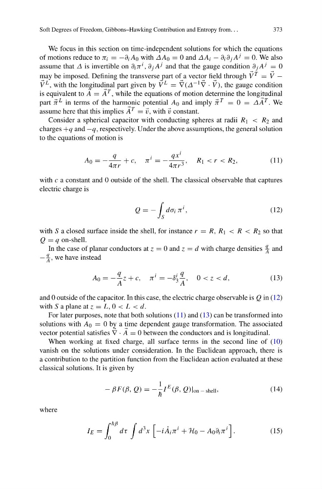
We focus in this section on time-independent solutions for which the equations
of motions reduce to π i = −∂ i A 0 with ΔA 0 = 0 and ΔA i − ∂ i ∂ j A j = 0. We also
assume that Δ is invertible on ∂ i π i , ∂ j A j and that the gauge condition ∂ j A j = 0
may be imposed. Defining the transverse part of a vector field through
V T =
V −
V L , with the longitudinal part given by
V L =
∇(Δ −1
∇ ·
V ), the gauge condition
is equivalent to
A =
A T , while the equations of motion determine the longitudinal
part
π L in terms of the harmonic potential A 0 and imply
π T = 0 = Δ
A T . We
assume here that this implies
A T = =
v, with
v constant.
Consider a spherical capacitor with conducting spheres at radii R 1 < R 2 and
charges +q and −q, respectively. Under the above assumptions, the general solution
to the equations of motion is
A 0 = −
q
4πr
+ c, π
i
= −
qx i
4πr 3 , R 1 < r < R 2 ,
(11)
with c a constant and 0 outside of the shell. The classical observable that captures
electric charge is
Q = −
S
dσ i π
i ,
(12)
with S a closed surface inside the shell, for instance r = R, R 1 < R < R 2 so that
Q = q on-shell.
In the case of planar conductors at z = 0 and z = d with charge densities
q
A and
−
q
A , we have instead
A 0 = −
q
A
z + c, π
i
= −δ
i
3
q
A
, 0 < z < d,
(13)
and 0 outside of the capacitor. In this case, the electric charge observable is Q in (12)
with S a plane at z = L, 0 < L < d.
For later purposes, note that both solutions (11) and (13) can be transformed into
solutions with A 0 = 0 by a time dependent gauge transformation. The associated
vector potential satisfies
∇ ·
A = 0 between the conductors and is longitudinal.
When working at fixed charge, all surface terms in the second line of (10)
vanish on the solutions under consideration. In the Euclidean approach, there is
a contribution to the partition function from the Euclidean action evaluated at these
classical solutions. It is given by
− βF (β, Q) = −
1
¯
h
I
E (β, Q)| on − shell ,
(14)
where
I E =
¯
hβ
0
dτ
d
3 x
−i ˙
A i π
i
+ H 0 − A 0 ∂ i π
i
.
(15)
373
We focus in this section on time-independent solutions for which the equations
of motions reduce to π i = −∂ i A 0 with ΔA 0 = 0 and ΔA i − ∂ i ∂ j A j = 0. We also
assume that Δ is invertible on ∂ i π i , ∂ j A j and that the gauge condition ∂ j A j = 0
may be imposed. Defining the transverse part of a vector field through
V T =
V −
V L , with the longitudinal part given by
V L =
∇(Δ −1
∇ ·
V ), the gauge condition
is equivalent to
A =
A T , while the equations of motion determine the longitudinal
part
π L in terms of the harmonic potential A 0 and imply
π T = 0 = Δ
A T . We
assume here that this implies
A T = =
v, with
v constant.
Consider a spherical capacitor with conducting spheres at radii R 1 < R 2 and
charges +q and −q, respectively. Under the above assumptions, the general solution
to the equations of motion is
A 0 = −
q
4πr
+ c, π
i
= −
qx i
4πr 3 , R 1 < r < R 2 ,
(11)
with c a constant and 0 outside of the shell. The classical observable that captures
electric charge is
Q = −
S
dσ i π
i ,
(12)
with S a closed surface inside the shell, for instance r = R, R 1 < R < R 2 so that
Q = q on-shell.
In the case of planar conductors at z = 0 and z = d with charge densities
q
A and
−
q
A , we have instead
A 0 = −
q
A
z + c, π
i
= −δ
i
3
q
A
, 0 < z < d,
(13)
and 0 outside of the capacitor. In this case, the electric charge observable is Q in (12)
with S a plane at z = L, 0 < L < d.
For later purposes, note that both solutions (11) and (13) can be transformed into
solutions with A 0 = 0 by a time dependent gauge transformation. The associated
vector potential satisfies
∇ ·
A = 0 between the conductors and is longitudinal.
When working at fixed charge, all surface terms in the second line of (10)
vanish on the solutions under consideration. In the Euclidean approach, there is
a contribution to the partition function from the Euclidean action evaluated at these
classical solutions. It is given by
− βF (β, Q) = −
1
¯
h
I
E (β, Q)| on − shell ,
(14)
where
I E =
¯
hβ
0
dτ
d
3 x
−i ˙
A i π
i
+ H 0 − A 0 ∂ i π
i
.
(15)