

298
K. Zelaya and V. Hussin
3 Point Transformation
In order to transform the Schrödinger equation of the stationary oscillator (2) into
the one of the nonstationary oscillator with time-dependent mass (7), let us consider
relationships between the elements of the set {y, τ, Ψ } and those of the set {x, t, ψ}
of the form [12]
y = y(x, t), τ = τ (x, t), Ψ = Ψ (y(x, t), τ (x, t)) = G(x, t; ψ(x, t)).
(8)
The dependence of Ψ on x and t is implicit, so, we have introduced the function
G as a reparametrization that allows to rewrite Ψ as an explicit function of x, t
and ψ. In this way, we have at hand a mechanism to map any solution of (2) into a
solution of (7). The explicit form of the relationships in (8) is determined through
the total derivatives
dΨ
dx ,
dΨ
dt and
d 2 Ψ
dx 2 . It allows finding relationships between the
partial derivative of the initial and final models, leading to the forms
∂Ψ
∂τ
= G 1
x, t; ψ,
∂ψ
∂x
,
∂ψ
∂t
,
∂ 2 Ψ
∂y 2 = G 2
x, t; ψ,
∂ψ
∂x
,
∂ 2 ψ
∂x 2 ,
∂ψ
∂t
.
(9)
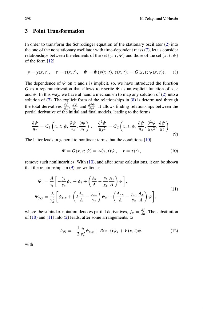
The latter leads in general to nonlinear terms, but the conditions [10]
Ψ = G(x, t; ψ) = A(x, t)ψ , τ = τ (t) ,
(10)
remove such nonlinearities. With (10), and after some calculations, it can be shown
that the relationships in (9) are written as
Ψ τ =
A
τ t
−
y t
y x
ψ x + ψ t +
A t
A
−
y t
y x
A x
A
ψ
,
Ψ y,y =
A
y 2
x
ψ x,x +
2
A x
A
−
y xx
y x
ψ x +
A xx
A
−
y xx
y x
A x
A
ψ
,
(11)
where the subindex notation denotes partial derivatives, f u =
∂f
∂u . The substitution
of (10) and (11) into (2) leads, after some arrangements, to
iψ t = −
1
2
τ t
y 2
x
ψ x,x + B(x, t)ψ x + V (x, t)ψ,
(12)
with
K. Zelaya and V. Hussin
3 Point Transformation
In order to transform the Schrödinger equation of the stationary oscillator (2) into
the one of the nonstationary oscillator with time-dependent mass (7), let us consider
relationships between the elements of the set {y, τ, Ψ } and those of the set {x, t, ψ}
of the form [12]
y = y(x, t), τ = τ (x, t), Ψ = Ψ (y(x, t), τ (x, t)) = G(x, t; ψ(x, t)).
(8)
The dependence of Ψ on x and t is implicit, so, we have introduced the function
G as a reparametrization that allows to rewrite Ψ as an explicit function of x, t
and ψ. In this way, we have at hand a mechanism to map any solution of (2) into a
solution of (7). The explicit form of the relationships in (8) is determined through
the total derivatives
dΨ
dx ,
dΨ
dt and
d 2 Ψ
dx 2 . It allows finding relationships between the
partial derivative of the initial and final models, leading to the forms
∂Ψ
∂τ
= G 1
x, t; ψ,
∂ψ
∂x
,
∂ψ
∂t
,
∂ 2 Ψ
∂y 2 = G 2
x, t; ψ,
∂ψ
∂x
,
∂ 2 ψ
∂x 2 ,
∂ψ
∂t
.
(9)
The latter leads in general to nonlinear terms, but the conditions [10]
Ψ = G(x, t; ψ) = A(x, t)ψ , τ = τ (t) ,
(10)
remove such nonlinearities. With (10), and after some calculations, it can be shown
that the relationships in (9) are written as
Ψ τ =
A
τ t
−
y t
y x
ψ x + ψ t +
A t
A
−
y t
y x
A x
A
ψ
,
Ψ y,y =
A
y 2
x
ψ x,x +
2
A x
A
−
y xx
y x
ψ x +
A xx
A
−
y xx
y x
A x
A
ψ
,
(11)
where the subindex notation denotes partial derivatives, f u =
∂f
∂u . The substitution
of (10) and (11) into (2) leads, after some arrangements, to
iψ t = −
1
2
τ t
y 2
x
ψ x,x + B(x, t)ψ x + V (x, t)ψ,
(12)
with