

240
R. Reyes et al.
The real case has been partially analyzed in the past, for factorization energies
coinciding with two consecutive energy levels of the initial Hamiltonian [13]. To
illustrate this example, let us take as seed solutions the two bound states associated
with the factorization energies 1 = E 2 and 2 = E 1 , which leads to the following
potential:
V 2 (x) =
(a + 2)(a + 3)
2
csc
2 (x) − b cot(x) + 4[(a + 3)
2
+ ˜
b
2
]
×
(a + 2) 2 + ˜
b 2 + [(a + 2)(a + 3) − ˜
b 2 ] cos(2x) − (2a + 5) ˜
b sin(2x)
{(a + 3) 2 + ˜
b 2 + [(a + 2)(a + 3) − ˜
b 2 ] cos(2x) − (2a + 5) ˜
b sin(2x)} 2
(14)
where ˜
b = b/(a + 1). Up to our knowledge, the explicit expression for this potential
is new.
Note that in this work we extend these results, by using general seed solutions (9)
whose factorization energies are not in the spectrum of the TRM potential. For doing
this, we need to choose carefully such seed solutions, since their behavior depends
on the two constants A, B involved in the linear combination (9), which will be
taken real in order to guarantee that the seed solutions will be real. Moreover, if
A, B have the same sign, then the number of zeros of the seed solution will be even,
otherwise it will be odd. This information is enough for selecting appropriately the
seed solutions, in order to implement non-singular transformations [10].
In Fig. 1 we can see several examples of how the new potential changes as the
spectrum of the TRM potential is modified by a second-order transformation in
the real case. In the left side we observe the potentials resulting from erasing two
consecutive energy levels (dotted and dashed curves) of V 0 (x) (continuous curve).
Let us note that the dashed curve in the graph corresponds to a potential given by
Eq. (14). On the right side of Fig. 1 it is seen the potentials resulting from adding
two levels in the same energy gap (dotted and dashed curves).
For the complex and confluent cases there exist some restrictions on the behavior
of the seed solutions at the edges of the x-domain (see for example [10–12]). As
the solutions (10) and (11) satisfy precisely such requirements, we can use them
directly to implement the corresponding transformations.
For two complex conjugate seed solutions, and factorization energies, the
implemented SUSY transformations generate isospectral potentials. Some examples
are shown in Fig. 2.
On the other hand, the confluent case generates Hamiltonians which can be
whether or not isospectral to the initial one. This depends on the w 0 -parameter of
Eq. (6), as well as of the factorization energy chosen. Due to the difficulty involved
in evaluating the integral for general factorization energies, in this work we show
only examples with a factorization energy coinciding with one of the energy levels
of the initial Hamiltonian. In Fig. 3 we can see examples of the new potentials
resulting from applying the confluent second-order SUSY transformation to the
TRM potentials for the two factorization energies 1 = E 0 , E 3 .
R. Reyes et al.
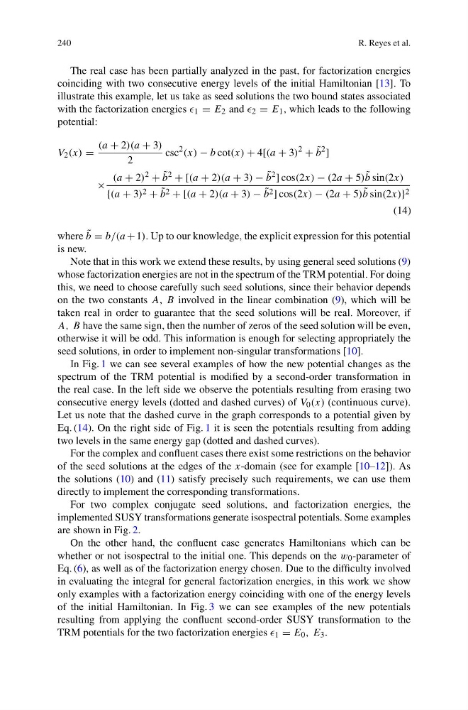
The real case has been partially analyzed in the past, for factorization energies
coinciding with two consecutive energy levels of the initial Hamiltonian [13]. To
illustrate this example, let us take as seed solutions the two bound states associated
with the factorization energies 1 = E 2 and 2 = E 1 , which leads to the following
potential:
V 2 (x) =
(a + 2)(a + 3)
2
csc
2 (x) − b cot(x) + 4[(a + 3)
2
+ ˜
b
2
]
×
(a + 2) 2 + ˜
b 2 + [(a + 2)(a + 3) − ˜
b 2 ] cos(2x) − (2a + 5) ˜
b sin(2x)
{(a + 3) 2 + ˜
b 2 + [(a + 2)(a + 3) − ˜
b 2 ] cos(2x) − (2a + 5) ˜
b sin(2x)} 2
(14)
where ˜
b = b/(a + 1). Up to our knowledge, the explicit expression for this potential
is new.
Note that in this work we extend these results, by using general seed solutions (9)
whose factorization energies are not in the spectrum of the TRM potential. For doing
this, we need to choose carefully such seed solutions, since their behavior depends
on the two constants A, B involved in the linear combination (9), which will be
taken real in order to guarantee that the seed solutions will be real. Moreover, if
A, B have the same sign, then the number of zeros of the seed solution will be even,
otherwise it will be odd. This information is enough for selecting appropriately the
seed solutions, in order to implement non-singular transformations [10].
In Fig. 1 we can see several examples of how the new potential changes as the
spectrum of the TRM potential is modified by a second-order transformation in
the real case. In the left side we observe the potentials resulting from erasing two
consecutive energy levels (dotted and dashed curves) of V 0 (x) (continuous curve).
Let us note that the dashed curve in the graph corresponds to a potential given by
Eq. (14). On the right side of Fig. 1 it is seen the potentials resulting from adding
two levels in the same energy gap (dotted and dashed curves).
For the complex and confluent cases there exist some restrictions on the behavior
of the seed solutions at the edges of the x-domain (see for example [10–12]). As
the solutions (10) and (11) satisfy precisely such requirements, we can use them
directly to implement the corresponding transformations.
For two complex conjugate seed solutions, and factorization energies, the
implemented SUSY transformations generate isospectral potentials. Some examples
are shown in Fig. 2.
On the other hand, the confluent case generates Hamiltonians which can be
whether or not isospectral to the initial one. This depends on the w 0 -parameter of
Eq. (6), as well as of the factorization energy chosen. Due to the difficulty involved
in evaluating the integral for general factorization energies, in this work we show
only examples with a factorization energy coinciding with one of the energy levels
of the initial Hamiltonian. In Fig. 3 we can see examples of the new potentials
resulting from applying the confluent second-order SUSY transformation to the
TRM potentials for the two factorization energies 1 = E 0 , E 3 .