

Supersymmetric Partners of the Rosen–Morse Potential
239
× 2 F 1
1−ν −a, −a−
iμ
2
; 2−ν −
iμ
2
; e
2ix
,
(10)
μ =
2b
E+
√
E 2 +b 2
,
ν= 1 −
E +
√
E 2 + b 2 ,
κ(a, ν, μ) =
Γ (2a+2)Γ (1−ν−i
μ
2 )
Γ (a+1−i
μ
2 )Γ (a+2−ν) , ρ(a, ν, μ) =
i
2
2a+1 Γ (2a+2)Γ (ν−1+i
μ
2 )
Γ (a+1+i
μ
2 )Γ (a+ν) ,
and
ψ R (x) = ψ L (π − x).
(11)
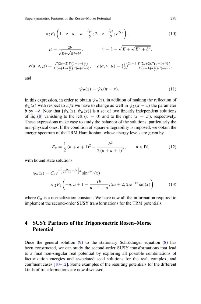
In this expression, in order to obtain ψ R (x), in addition of making the reflection of
ψ L (x) with respect to π/2 we have to change as well in ψ L (π − x) the parameter
b by −b. Note that {ψ L (x), ψ R (x)} is a set of two linearly independent solutions
of Eq. (8) vanishing to the left (x = 0) and to the right (x = π ), respectively.
These expressions make easy to study the behavior of the solutions, particularly the
non-physical ones. If the condition of square-integrability is imposed, we obtain the
energy spectrum of the TRM Hamiltonian, whose energy levels are given by
E n =
1
2
(n + a + 1)
2
−
b 2
2 (n + a + 1)
2
,
n∈ IN,
(12)
with bound state solutions
ψ n (x) = C n e
−
b
n+1+a −in
x sin
a+1 (x)
× 2 F 1
−n, a + 1 −
ib
n + 1 + a
; 2a + 2; 2ie
−ix sin(x)
,
(13)
where C n is a normalization constant. We have now all the information required to
implement the second-order SUSY transformations for the TRM potentials.
4 SUSY Partners of the Trigonometric Rosen–Morse
Potential
Once the general solution (9) to the stationary Schrödinger equation (8) has
been constructed, we can study the second-order SUSY transformations that lead
to a final non-singular real potential by exploring all possible combinations of
factorization energies and associated seed solutions for the real, complex, and
confluent cases [10–12]. Some examples of the resulting potentials for the different
kinds of transformations are now discussed.
239
× 2 F 1
1−ν −a, −a−
iμ
2
; 2−ν −
iμ
2
; e
2ix
,
(10)
μ =
2b
E+
√
E 2 +b 2
,
ν= 1 −
E +
√
E 2 + b 2 ,
κ(a, ν, μ) =
Γ (2a+2)Γ (1−ν−i
μ
2 )
Γ (a+1−i
μ
2 )Γ (a+2−ν) , ρ(a, ν, μ) =
i
2
2a+1 Γ (2a+2)Γ (ν−1+i
μ
2 )
Γ (a+1+i
μ
2 )Γ (a+ν) ,
and
ψ R (x) = ψ L (π − x).
(11)
In this expression, in order to obtain ψ R (x), in addition of making the reflection of
ψ L (x) with respect to π/2 we have to change as well in ψ L (π − x) the parameter
b by −b. Note that {ψ L (x), ψ R (x)} is a set of two linearly independent solutions
of Eq. (8) vanishing to the left (x = 0) and to the right (x = π ), respectively.
These expressions make easy to study the behavior of the solutions, particularly the
non-physical ones. If the condition of square-integrability is imposed, we obtain the
energy spectrum of the TRM Hamiltonian, whose energy levels are given by
E n =
1
2
(n + a + 1)
2
−
b 2
2 (n + a + 1)
2
,
n∈ IN,
(12)
with bound state solutions
ψ n (x) = C n e
−
b
n+1+a −in
x sin
a+1 (x)
× 2 F 1
−n, a + 1 −
ib
n + 1 + a
; 2a + 2; 2ie
−ix sin(x)
,
(13)
where C n is a normalization constant. We have now all the information required to
implement the second-order SUSY transformations for the TRM potentials.
4 SUSY Partners of the Trigonometric Rosen–Morse
Potential
Once the general solution (9) to the stationary Schrödinger equation (8) has
been constructed, we can study the second-order SUSY transformations that lead
to a final non-singular real potential by exploring all possible combinations of
factorization energies and associated seed solutions for the real, complex, and
confluent cases [10–12]. Some examples of the resulting potentials for the different
kinds of transformations are now discussed.