6
F. Finkel et al.
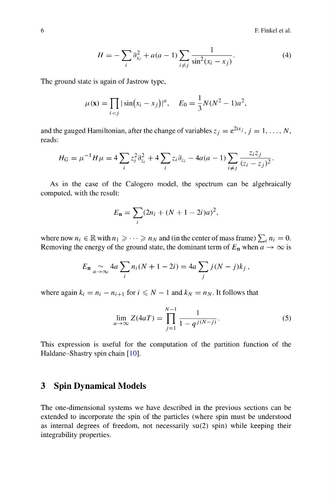
H = −
i
∂
2
x i
+ a(a − 1)
i =j
1
sin
2 (x i − x j )
.
(4)
The ground state is again of Jastrow type,
μ(x) =
i | sin
x i − x j
|
a , E 0 =
1
3
N(N
2
− 1)a
2 ,
and the gauged Hamiltonian, after the change of variables z j = e 2ix j , j = 1, . . . , N,
reads:
H G = μ
−1 H μ = 4
i
z
2
i ∂
2
z i
+ 4
i
z i ∂ z i − 4a(a − 1)
i =j
z i z j
(z i − z j ) 2 .
As in the case of the Calogero model, the spectrum can be algebraically
computed, with the result:
E n =
i
(2n i + (N + 1 − 2i)a)
2 ,
where now n i ∈ R with n 1 · · · n N and (in the center of mass frame)
i n i = 0.
Removing the energy of the ground state, the dominant term of E n when a → ∞ is
E n ∼
a→∞
4a
i
n i (N + 1 − 2i) = 4a
j
j (N − j)k j ,
where again k i = n i − n i+1 for i N − 1 and k N = n N . It follows that
lim
a→∞
Z(4aT ) =
N −1
j =1
1
1 − q j (N−j) .
(5)
This expression is useful for the computation of the partition function of the
Haldane–Shastry spin chain [10].
3 Spin Dynamical Models
The one-dimensional systems we have described in the previous sections can be
extended to incorporate the spin of the particles (where spin must be understood
as internal degrees of freedom, not necessarily su(2) spin) while keeping their
integrability properties.