

572
M. Saini et al.
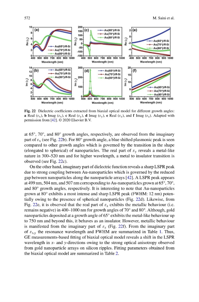
Fig. 22 Dielectric coefficients extracted from biaxial optical model for different growth angles:
a Real (ε x ), b Imag (ε x ), c Real (ε y ), d Imag (ε y ), e Real (ε z ), and f Imag (ε z ). Adapted with
permission from [42]. © 2020 Elsevier B.V.
at 65°, 70°, and 80° growth angles, respectively, are observed from the imaginary
part of ε x (see Fig. 22b). For 80° growth angle, a blue shifted plasmonic peak is seen
compared to other growth angles which is governed by the transition in the shape
(elongated to spherical) of nanoparticles. The real part of ε y reveals a metal-like
nature in 300–520 nm and for higher wavelength, a metal to insulator transition is
observed (see Fig. 22c).
On the other hand, imaginary part of dielectric function reveals a sharp LSPR peak
due to strong coupling between Au-nanoparticles which is governed by the reduced
gap between nanoparticles along the nanoparticle arrays [42]. A LSPR peak appears
at 499 nm, 504 nm, and 507 nm corresponding to Au-nanoparticles grown at 65°, 70°,
and 80° growth angles, respectively. It is interesting to note that Au-nanoparticles
grown at 80° exhibits a most intense and sharp LSPR peak (FWHM: 12 nm) potentially owing to the presence of spherical nanoparticles (Fig. 22d). Likewise, from
Fig. 22e, it is observed that the real part of ε z exhibits the metallic behaviour (i.e.
remains negative) in 400–1000 nm for growth angles of 70° and 80°. Although, gold
nanoparticles deposited at a growth angle of 65° exhibits the metal-like behaviour up
to 750 nm and beyond this, it behaves as an insulator. However, metallic behaviour
is manifested from the imaginary part of ε z (Fig. 22f). From the imaginary part
of ε x,y the resonance wavelength and FWHM are summarized in Table 1. Thus,
GE measurements-based fitting of biaxial optical model reveals a shift in the LSPR
wavelength in x- and y-directions owing to the strong optical anisotropy observed
from gold nanoparticle arrays on silicon ripples. Fitting parameters obtained from
the biaxial optical model are summarized in Table 2.
M. Saini et al.
Fig. 22 Dielectric coefficients extracted from biaxial optical model for different growth angles:
a Real (ε x ), b Imag (ε x ), c Real (ε y ), d Imag (ε y ), e Real (ε z ), and f Imag (ε z ). Adapted with
permission from [42]. © 2020 Elsevier B.V.
at 65°, 70°, and 80° growth angles, respectively, are observed from the imaginary
part of ε x (see Fig. 22b). For 80° growth angle, a blue shifted plasmonic peak is seen
compared to other growth angles which is governed by the transition in the shape
(elongated to spherical) of nanoparticles. The real part of ε y reveals a metal-like
nature in 300–520 nm and for higher wavelength, a metal to insulator transition is
observed (see Fig. 22c).
On the other hand, imaginary part of dielectric function reveals a sharp LSPR peak
due to strong coupling between Au-nanoparticles which is governed by the reduced
gap between nanoparticles along the nanoparticle arrays [42]. A LSPR peak appears
at 499 nm, 504 nm, and 507 nm corresponding to Au-nanoparticles grown at 65°, 70°,
and 80° growth angles, respectively. It is interesting to note that Au-nanoparticles
grown at 80° exhibits a most intense and sharp LSPR peak (FWHM: 12 nm) potentially owing to the presence of spherical nanoparticles (Fig. 22d). Likewise, from
Fig. 22e, it is observed that the real part of ε z exhibits the metallic behaviour (i.e.
remains negative) in 400–1000 nm for growth angles of 70° and 80°. Although, gold
nanoparticles deposited at a growth angle of 65° exhibits the metal-like behaviour up
to 750 nm and beyond this, it behaves as an insulator. However, metallic behaviour
is manifested from the imaginary part of ε z (Fig. 22f). From the imaginary part
of ε x,y the resonance wavelength and FWHM are summarized in Table 1. Thus,
GE measurements-based fitting of biaxial optical model reveals a shift in the LSPR
wavelength in x- and y-directions owing to the strong optical anisotropy observed
from gold nanoparticle arrays on silicon ripples. Fitting parameters obtained from
the biaxial optical model are summarized in Table 2.