

Impedance Spectroscopy
531
Fig. 6 Schematic representation of frequency dependence of permittivity for planar and homeotropically aligned liquid crystalline molecules showing several possible relaxation mechanisms
ε
∗
= ε(∞) +
δε k
1 + ( j f τ k )
α k
β k +
A
f n − j
σ i
ε 0 ω s − j B f
m
(20)
where k indicates the number of relaxation processes. δε k , τ k , α k and β k are the
dielectric increment, relaxation time, symmetric and asymmetric parameters for the
k
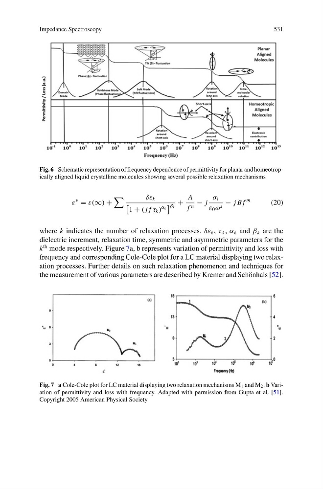
th mode respectively. Figure 7a, b represents variation of permittivity and loss with
frequency and corresponding Cole-Cole plot for a LC material displaying two relaxation processes. Further details on such relaxation phenomenon and techniques for
the measurement of various parameters are described by Kremer and Schönhals [52].
Fig. 7 a Cole-Cole plot for LC material displaying two relaxation mechanisms M 1 and M 2 . b Variation of permittivity and loss with frequency. Adapted with permission from Gupta et al. [51].
Copyright 2005 American Physical Society
531
Fig. 6 Schematic representation of frequency dependence of permittivity for planar and homeotropically aligned liquid crystalline molecules showing several possible relaxation mechanisms
ε
∗
= ε(∞) +
δε k
1 + ( j f τ k )
α k
β k +
A
f n − j
σ i
ε 0 ω s − j B f
m
(20)
where k indicates the number of relaxation processes. δε k , τ k , α k and β k are the
dielectric increment, relaxation time, symmetric and asymmetric parameters for the
k
th mode respectively. Figure 7a, b represents variation of permittivity and loss with
frequency and corresponding Cole-Cole plot for a LC material displaying two relaxation processes. Further details on such relaxation phenomenon and techniques for
the measurement of various parameters are described by Kremer and Schönhals [52].
Fig. 7 a Cole-Cole plot for LC material displaying two relaxation mechanisms M 1 and M 2 . b Variation of permittivity and loss with frequency. Adapted with permission from Gupta et al. [51].
Copyright 2005 American Physical Society