

Impedance Spectroscopy
529
ε
∗
= ε(∞) +
δε
1 + ( j f τ )
(1−α)
(17)
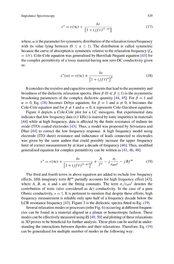
where, α is the parameter for symmetric distribution of the relaxation times/frequency
with its value lying between (0 ≤ α ≤ 1). The distribution is called symmetric
because the curve of absorption is symmetric relative to the relaxation frequency (f R
= 1/τ ). Cole-Cole equation was generalised by Havriliak-Negami equation [43] for
the complex permittivity of a lossy material having non zero DC conductivity given
as:
ε
∗
(ω) = ε(∞) +
δε
1 + ( j f τ )
α
β
(18)
It considers the resistive and capacitive components that lead to the asymmetry and
broadness of the dielectric relaxation spectra. Here β (0 β ≤ 1) is the asymmetric
broadening parameters of the complex dielectric quantity [44, 45]. For β = 1 and
α = 0, Eq. (18) becomes Debye equation; for β = 1 and α = 0, it becomes the
Cole-Cole equation and for β = 1 and α = 0, it represents Cole-Davidson equation.
Figure 4 depicts a Cole-Cole plot for a LC mesogens. But experimental data
indicates that low frequency data (<1 kHz) is marred by ionic impurities in materials
[44] while at high frequency, data is affected by the finite resistance of indium tin
oxide (ITO) coated electrodes [43]. Thus, a model was proposed by Srivastava and
Dhar [44] to correct the low frequency response. A high frequency model using
electrode (ITO sheet) resistance and inductance of leads connected to electrodes
was given by the same author that could possibly increase the upper frequency
limit of correct measurement by at least a decade of frequency [46]. Thus, modified
generalised equation for complex permittivity can be written as [41, 46, 48]:
ε
∗
= ε(∞) +
δε
1 + ( j f τ )
(1−α)
β +
A
f n − j
σ i
ε 0 ω s − j B f
m
(19)
The third and fourth terms in above equation are added to include low frequency
effects, fifth imaginary term Bf
m partially accounts for high frequency effect [43],
where A, B, m, n and s are the fitting constants. The term σ i /ε 0 ω
s denotes the
contribution of ionic (also considered as dc) conductivity. In the case of a pure
Ohmic conductivity, s = 1. It is pertinent to mention that despite these efforts, high
frequency measurement is reliable only upto half of a frequency decade below the
LCR resonance frequency [43]. Figure 5 is the dielectric spectra fitted to Eq. (19).
Several relaxation modes or processes (refer Fig. 6) occurring at different frequencies can be found in a material aligned in a planar or homeotropic fashion. These
modes can be effectively measured using IS [49, 50] and plotting of these relaxations
in 3D proves to be beneficial for further analysis. These plots can be useful in understanding the interactions between dipoles and their relaxations. Therefore, Eq. (19)
can be generalized for multiple number of modes in the following way:
529
ε
∗
= ε(∞) +
δε
1 + ( j f τ )
(1−α)
(17)
where, α is the parameter for symmetric distribution of the relaxation times/frequency
with its value lying between (0 ≤ α ≤ 1). The distribution is called symmetric
because the curve of absorption is symmetric relative to the relaxation frequency (f R
= 1/τ ). Cole-Cole equation was generalised by Havriliak-Negami equation [43] for
the complex permittivity of a lossy material having non zero DC conductivity given
as:
ε
∗
(ω) = ε(∞) +
δε
1 + ( j f τ )
α
β
(18)
It considers the resistive and capacitive components that lead to the asymmetry and
broadness of the dielectric relaxation spectra. Here β (0 β ≤ 1) is the asymmetric
broadening parameters of the complex dielectric quantity [44, 45]. For β = 1 and
α = 0, Eq. (18) becomes Debye equation; for β = 1 and α = 0, it becomes the
Cole-Cole equation and for β = 1 and α = 0, it represents Cole-Davidson equation.
Figure 4 depicts a Cole-Cole plot for a LC mesogens. But experimental data
indicates that low frequency data (<1 kHz) is marred by ionic impurities in materials
[44] while at high frequency, data is affected by the finite resistance of indium tin
oxide (ITO) coated electrodes [43]. Thus, a model was proposed by Srivastava and
Dhar [44] to correct the low frequency response. A high frequency model using
electrode (ITO sheet) resistance and inductance of leads connected to electrodes
was given by the same author that could possibly increase the upper frequency
limit of correct measurement by at least a decade of frequency [46]. Thus, modified
generalised equation for complex permittivity can be written as [41, 46, 48]:
ε
∗
= ε(∞) +
δε
1 + ( j f τ )
(1−α)
β +
A
f n − j
σ i
ε 0 ω s − j B f
m
(19)
The third and fourth terms in above equation are added to include low frequency
effects, fifth imaginary term Bf
m partially accounts for high frequency effect [43],
where A, B, m, n and s are the fitting constants. The term σ i /ε 0 ω
s denotes the
contribution of ionic (also considered as dc) conductivity. In the case of a pure
Ohmic conductivity, s = 1. It is pertinent to mention that despite these efforts, high
frequency measurement is reliable only upto half of a frequency decade below the
LCR resonance frequency [43]. Figure 5 is the dielectric spectra fitted to Eq. (19).
Several relaxation modes or processes (refer Fig. 6) occurring at different frequencies can be found in a material aligned in a planar or homeotropic fashion. These
modes can be effectively measured using IS [49, 50] and plotting of these relaxations
in 3D proves to be beneficial for further analysis. These plots can be useful in understanding the interactions between dipoles and their relaxations. Therefore, Eq. (19)
can be generalized for multiple number of modes in the following way: