

Fluorescence Spectrometry
453
The Lippert-Mataga equation represents an approximation and is applicable if
the specific interactions such as conformational changes are not present. If hydrogen
bonds formation takes place between the solute-solvent, this equation can not be
used. In general, it can be used under the reorganization of the electronic levels that
can result in different LUMO (Lowest Unoccupied Molecular Orbital) levels of different solvents. Sometimes the solvatochromic blue shift is observed with increasing
solvent-polarity that is exclusively attributed to geometric effect. The Lippert-Mataga
relation does not include such geometric effects and therefore, couldn’t predict a
blueshift. Under the influence of these critical points, the emission spectrum is found
to shift depending upon the net polarity of the solvent, magnitude of local interactions
and change in relaxation time scale.
2.3.3 Effect of Impurities
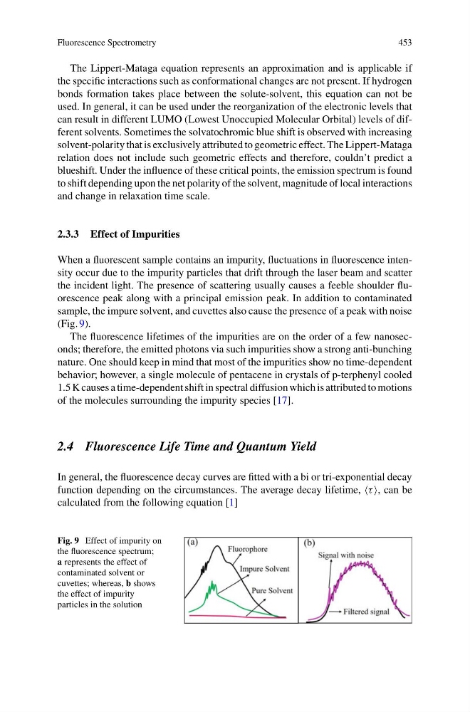
When a fluorescent sample contains an impurity, fluctuations in fluorescence intensity occur due to the impurity particles that drift through the laser beam and scatter
the incident light. The presence of scattering usually causes a feeble shoulder fluorescence peak along with a principal emission peak. In addition to contaminated
sample, the impure solvent, and cuvettes also cause the presence of a peak with noise
(Fig. 9).
The fluorescence lifetimes of the impurities are on the order of a few nanoseconds; therefore, the emitted photons via such impurities show a strong anti-bunching
nature. One should keep in mind that most of the impurities show no time-dependent
behavior; however, a single molecule of pentacene in crystals of p-terphenyl cooled
1.5 K causes a time-dependent shift in spectral diffusion which is attributed to motions
of the molecules surrounding the impurity species [17].
2.4 Fluorescence Life Time and Quantum Yield
In general, the fluorescence decay curves are fitted with a bi or tri-exponential decay
function depending on the circumstances. The average decay lifetime, τ , can be
calculated from the following equation [1]
Fig. 9 Effect of impurity on
the fluorescence spectrum;
a represents the effect of
contaminated solvent or
cuvettes; whereas, b shows
the effect of impurity
particles in the solution
453
The Lippert-Mataga equation represents an approximation and is applicable if
the specific interactions such as conformational changes are not present. If hydrogen
bonds formation takes place between the solute-solvent, this equation can not be
used. In general, it can be used under the reorganization of the electronic levels that
can result in different LUMO (Lowest Unoccupied Molecular Orbital) levels of different solvents. Sometimes the solvatochromic blue shift is observed with increasing
solvent-polarity that is exclusively attributed to geometric effect. The Lippert-Mataga
relation does not include such geometric effects and therefore, couldn’t predict a
blueshift. Under the influence of these critical points, the emission spectrum is found
to shift depending upon the net polarity of the solvent, magnitude of local interactions
and change in relaxation time scale.
2.3.3 Effect of Impurities
When a fluorescent sample contains an impurity, fluctuations in fluorescence intensity occur due to the impurity particles that drift through the laser beam and scatter
the incident light. The presence of scattering usually causes a feeble shoulder fluorescence peak along with a principal emission peak. In addition to contaminated
sample, the impure solvent, and cuvettes also cause the presence of a peak with noise
(Fig. 9).
The fluorescence lifetimes of the impurities are on the order of a few nanoseconds; therefore, the emitted photons via such impurities show a strong anti-bunching
nature. One should keep in mind that most of the impurities show no time-dependent
behavior; however, a single molecule of pentacene in crystals of p-terphenyl cooled
1.5 K causes a time-dependent shift in spectral diffusion which is attributed to motions
of the molecules surrounding the impurity species [17].
2.4 Fluorescence Life Time and Quantum Yield
In general, the fluorescence decay curves are fitted with a bi or tri-exponential decay
function depending on the circumstances. The average decay lifetime, τ , can be
calculated from the following equation [1]
Fig. 9 Effect of impurity on
the fluorescence spectrum;
a represents the effect of
contaminated solvent or
cuvettes; whereas, b shows
the effect of impurity
particles in the solution