

264
P. Madhusudhan et al.
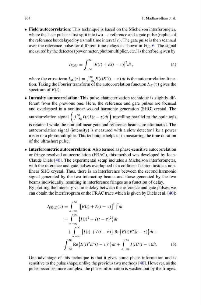
• Field autocorrelation: This technique is based on the Michelson interferometer,
where the laser pulse is first split into two—a reference and a gate pulse (replica of
the reference but delayed by a small time interval τ ). The gate pulse is then scanned
over the reference pulse for different time delays as shown in Fig. 6. The signal
measured by the detector (power meter, photomultiplier, etc.) is therefore, given by
I Field =
∞
−∞
E(t) + E(t − τ )
2 dt ,
(4)
where the cross-term I AC (τ ) =
∞
−∞ E(t)E
∗
(t − τ ) dt is the autocorrelation function. Taking the Fourier transform of the autocorrelation function I AC (τ ) gives the
spectrum of E(t).
• Intensity autocorrelation: This pulse characterization technique is slightly different from the previous one. Here, the reference and gate pulses are focused
and overlapped in a nonlinear second harmonic generation (SHG) crystal. The
autocorrelation signal
∞
−∞ I (t)I (t − τ )dt
travelling parallel to the optic axis
is retained while the non-collinear gate and reference beams are eliminated. The
autocorrelation signal (intensity) is measured with a slow detector like a power
meter or a photomultiplier. This technique helps us in measuring the time duration
of the ultrashort pulse.
• Interferometric autocorrelation: Also termed as phase-sensitive autocorrelation
or fringe-resolved autocorrelation (FRAC), this method was developed by JeanClaude Diels [40]. The experimental setup includes a Michelson interferometer,
with the reference and gate pulses overlapped in a collinear fashion inside a nonlinear SHG crystal. Thus, there is an interference between the second harmonic
signal generated by the two interacting beams and those generated by the two
beams individually, resulting in interference fringes as a function of delay.
By plotting the intensity vs time delay between the reference and gate pulses, we
can obtain the interferogram or the FRAC trace which is given by Diels et al. [40]:
I FRAC (τ ) =
∞
−∞
E(t) + E(t − τ )
2
2 dt
=
∞
−∞
I (t)
2
+ I (t − τ )
2
dt
+
∞
−∞
I (t) + I (t − τ )
Re
E(t)E
∗
(t − τ )
dt +
∞
−∞
Re
E(t)
2 E
∗
(t − τ )
2
dt +
∞
−∞
I (t)I (t − τ )dt.
(5)
One advantage of this technique is that it gives some phase information and is
sensitive to the pulse shape, unlike the previous two methods [40]. However, as the
pulse becomes more complex, the phase information is washed out by the fringes.
P. Madhusudhan et al.
• Field autocorrelation: This technique is based on the Michelson interferometer,
where the laser pulse is first split into two—a reference and a gate pulse (replica of
the reference but delayed by a small time interval τ ). The gate pulse is then scanned
over the reference pulse for different time delays as shown in Fig. 6. The signal
measured by the detector (power meter, photomultiplier, etc.) is therefore, given by
I Field =
∞
−∞
E(t) + E(t − τ )
2 dt ,
(4)
where the cross-term I AC (τ ) =
∞
−∞ E(t)E
∗
(t − τ ) dt is the autocorrelation function. Taking the Fourier transform of the autocorrelation function I AC (τ ) gives the
spectrum of E(t).
• Intensity autocorrelation: This pulse characterization technique is slightly different from the previous one. Here, the reference and gate pulses are focused
and overlapped in a nonlinear second harmonic generation (SHG) crystal. The
autocorrelation signal
∞
−∞ I (t)I (t − τ )dt
travelling parallel to the optic axis
is retained while the non-collinear gate and reference beams are eliminated. The
autocorrelation signal (intensity) is measured with a slow detector like a power
meter or a photomultiplier. This technique helps us in measuring the time duration
of the ultrashort pulse.
• Interferometric autocorrelation: Also termed as phase-sensitive autocorrelation
or fringe-resolved autocorrelation (FRAC), this method was developed by JeanClaude Diels [40]. The experimental setup includes a Michelson interferometer,
with the reference and gate pulses overlapped in a collinear fashion inside a nonlinear SHG crystal. Thus, there is an interference between the second harmonic
signal generated by the two interacting beams and those generated by the two
beams individually, resulting in interference fringes as a function of delay.
By plotting the intensity vs time delay between the reference and gate pulses, we
can obtain the interferogram or the FRAC trace which is given by Diels et al. [40]:
I FRAC (τ ) =
∞
−∞
E(t) + E(t − τ )
2
2 dt
=
∞
−∞
I (t)
2
+ I (t − τ )
2
dt
+
∞
−∞
I (t) + I (t − τ )
Re
E(t)E
∗
(t − τ )
dt +
∞
−∞
Re
E(t)
2 E
∗
(t − τ )
2
dt +
∞
−∞
I (t)I (t − τ )dt.
(5)
One advantage of this technique is that it gives some phase information and is
sensitive to the pulse shape, unlike the previous two methods [40]. However, as the
pulse becomes more complex, the phase information is washed out by the fringes.