

Modern Experimental Techniques in Ultrafast Atomic …
263
intensity of the field
∞
−∞
E(t)
2 dt
. They do not give any information about the
temporal or spectral phase.
An ultrashort pulse is mathematically represented as
E(t) =
I (t)e
i(ω 0 t−φ(t))
,
(1)
where I is the intensity, ω 0 is the central frequency and φ(t) is the phase. The above
equation can be written in the frequency domain as
E(ω) =
S(ω − ω 0 )e
i(φ(ω−ω 0 ))
,
(2)
where S(ω) is the spectrum of the pulse, and φ(ω) is the spectral phase. The
spectral phase is related to the instantaneous frequency ω(t) as
ω(t) = ω 0 −
d φ
dt
.
(3)
Let us first take a look at the primeval techniques of ultrashort pulse characterization, before moving on to the latest characterization techniques.
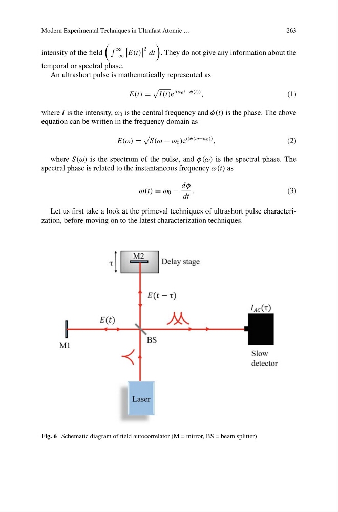
Fig. 6 Schematic diagram of field autocorrelator (M = mirror, BS = beam splitter)
263
intensity of the field
∞
−∞
E(t)
2 dt
. They do not give any information about the
temporal or spectral phase.
An ultrashort pulse is mathematically represented as
E(t) =
I (t)e
i(ω 0 t−φ(t))
,
(1)
where I is the intensity, ω 0 is the central frequency and φ(t) is the phase. The above
equation can be written in the frequency domain as
E(ω) =
S(ω − ω 0 )e
i(φ(ω−ω 0 ))
,
(2)
where S(ω) is the spectrum of the pulse, and φ(ω) is the spectral phase. The
spectral phase is related to the instantaneous frequency ω(t) as
ω(t) = ω 0 −
d φ
dt
.
(3)
Let us first take a look at the primeval techniques of ultrashort pulse characterization, before moving on to the latest characterization techniques.
Fig. 6 Schematic diagram of field autocorrelator (M = mirror, BS = beam splitter)