

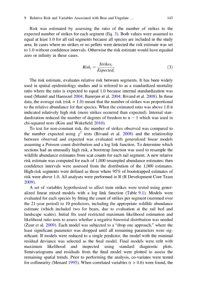
Risk was estimated by assessing the ratio of the number of strikes to the
expected number of strikes for each segment (Eq. 3). Both values were assumed to
equal at least 1.0 for all rail segments because all species are included in the study
area. In cases where no strikes or no pellets were detected the risk estimate was set
to 1.0 without confidence intervals. Otherwise the risk estimate would have equaled
zero or infinity in these cases.
Risk i ¼
Strikes i
Expected i
ð3Þ
The risk estimate, evaluates relative risk between segments. It has been widely
used in spatial epidemiology studies and is referred to as a standardized mortality
ratio where the ratio is expected to equal 1.0 because internal standardization was
used (Mantel and Haenszel 2004; Banerjee et al. 2004; Bivand et al. 2008). In these
data, the average risk (risk = 1.0) meant that the number of strikes was proportional
to the relative abundance for that species. When the estimated ratio was above 1.0 it
indicated relatively high risk (more strikes occurred than expected). Internal standardization reduced the number of degrees of freedom to n − 1 which was used in
chi-squared tests (Kim and Wakefield 2010).
To test for non-constant risk, the number of strikes observed was compared to
the number expected using v
2 tests (Bivand et al. 2008) and the relationship
between observed and expected was evaluated with generalized linear models
assuming a Poisson count distribution and a log link function. To determine which
sections had an unusually high risk, a bootstrap function was used to resample the
wildlife abundance estimates from scat counts for each rail segment. A new relative
risk estimate was computed for each of 1,000 resampled abundance estimates; then
confidence intervals were assessed from the distribution of the 1,000 estimates.
High-risk segments were defined as those where 95% of bootstrapped estimates of
risk were above 1.0. All analyses were performed in R (R Development Core Team
2009).
A set of variables hypothesized to affect train strikes were tested using generalized linear mixed models with a log link function (Table 9.1). Models were
evaluated for each species by fitting the count of strikes per segment (summed over
the 21-year period) to 10 predictors, including the appropriate wildlife abundance
estimate (which included two for bears, due to evaluation at the rail bed and
landscape scales). Initial fits used restricted maximum likelihood estimation and
likelihood ratio tests to assess whether a negative binomial distribution was needed
(Zuur et al. 2009). Each model was subjected to a “drop one approach,” where the
least significant parameter was dropped until all remaining parameters were significant. If models were reduced to a single predictor, the model with the minimal
residual deviance was selected as the final model. Final models were refit with
maximum likelihood and inspected using standard diagnostic plots.
Semivariograms and residuals from the final model were plotted to assess the
remaining spatial trends. Prior to performing the analysis, co-variates were tested
for collinearity (Menard 1995). When correlated variables (r > 0.6) were found, the
9 Relative Risk and Variables Associated with Bear and Ungulate …
143
expected number of strikes for each segment (Eq. 3). Both values were assumed to
equal at least 1.0 for all rail segments because all species are included in the study
area. In cases where no strikes or no pellets were detected the risk estimate was set
to 1.0 without confidence intervals. Otherwise the risk estimate would have equaled
zero or infinity in these cases.
Risk i ¼
Strikes i
Expected i
ð3Þ
The risk estimate, evaluates relative risk between segments. It has been widely
used in spatial epidemiology studies and is referred to as a standardized mortality
ratio where the ratio is expected to equal 1.0 because internal standardization was
used (Mantel and Haenszel 2004; Banerjee et al. 2004; Bivand et al. 2008). In these
data, the average risk (risk = 1.0) meant that the number of strikes was proportional
to the relative abundance for that species. When the estimated ratio was above 1.0 it
indicated relatively high risk (more strikes occurred than expected). Internal standardization reduced the number of degrees of freedom to n − 1 which was used in
chi-squared tests (Kim and Wakefield 2010).
To test for non-constant risk, the number of strikes observed was compared to
the number expected using v
2 tests (Bivand et al. 2008) and the relationship
between observed and expected was evaluated with generalized linear models
assuming a Poisson count distribution and a log link function. To determine which
sections had an unusually high risk, a bootstrap function was used to resample the
wildlife abundance estimates from scat counts for each rail segment. A new relative
risk estimate was computed for each of 1,000 resampled abundance estimates; then
confidence intervals were assessed from the distribution of the 1,000 estimates.
High-risk segments were defined as those where 95% of bootstrapped estimates of
risk were above 1.0. All analyses were performed in R (R Development Core Team
2009).
A set of variables hypothesized to affect train strikes were tested using generalized linear mixed models with a log link function (Table 9.1). Models were
evaluated for each species by fitting the count of strikes per segment (summed over
the 21-year period) to 10 predictors, including the appropriate wildlife abundance
estimate (which included two for bears, due to evaluation at the rail bed and
landscape scales). Initial fits used restricted maximum likelihood estimation and
likelihood ratio tests to assess whether a negative binomial distribution was needed
(Zuur et al. 2009). Each model was subjected to a “drop one approach,” where the
least significant parameter was dropped until all remaining parameters were significant. If models were reduced to a single predictor, the model with the minimal
residual deviance was selected as the final model. Final models were refit with
maximum likelihood and inspected using standard diagnostic plots.
Semivariograms and residuals from the final model were plotted to assess the
remaining spatial trends. Prior to performing the analysis, co-variates were tested
for collinearity (Menard 1995). When correlated variables (r > 0.6) were found, the
9 Relative Risk and Variables Associated with Bear and Ungulate …
143