

2011). Therefore, grain density was weighted by the week of year it was measured. For
both years, the weighted value was calculated as the mean seed count multiplied by the
average rate of decrease (3%) for each additional week after April 15th (data not
shown). For example, a weighted seed count of 80 wheat and barley seeds measured
on June 20th (4 weeks after April 15th) was [80 Â (0.97 Â 4) = 310.4]. The grain
density data were binned to the appropriate 4.86 km long segment in a GIS.
The GIS layer representing the railroad contained additional information on train
speed limits, bridges, sidings and track grades. The highest posted train speed limit
(SPEED max ) and mean track grade (GRADE mean ) were calculated for each segment.
The variable SINUOSITY was calculated using the “sinuosity” function in Hawth’s
analysis tools extension for ArcGIS 9 (ESRI Redlands, CA 2004). The number of
bridges were counted and summed for the variable, hereinafter termed “BRIDGE c ”.
A count of vehicle overpasses, tunnels, snow sheds or rock cuts occurring along each
segment were each given a value of “1” and summed for the variable hereinafter called
“BARRIER c ”. The lengths of track inside two tunnels and one secondary track west of
Lake Louise were omitted from analyses; in all, 28 segments were used in the analysis.
Data Analysis
Analyses were conducted independently for elk, deer and bears. Strikes that occurred
over the 21-year period were compared to relative abundance estimated using data
covering a 2-year period (2008 and 2009). This comparison assumes that relative
abundance across the study area remained relatively stable during the preceding
years. To assess this assumption, we looked for changes in the distribution of strikes
over time. A better approach would be to assess changes in relative abundance over
time, but these data were not available for enough of the study area or species.
Changes in the distribution of strikes over time were assessed by conducting
ANOVA on year and rail segments. More variability in year than rail segment may
mean that substantial shifts occurred in the relative abundance, therby invalidating
further analysis. Next, to determine if strikes and/or wildlife abundance were evenly
distributed along the CPR, chi-squared tests were used. To identify hotspots the
upper 95% confidence interval of strikes per segment was used, which assumed that
the counts followed a Poisson distribution (Bivand et al. 2008; Malo et al. 2004).
Risk estimates for each rail segment were developed through three steps. First,
the RA rail corridor or RA rail bed estimates for each segment (i) were converted to a
percentage of the total from all rail segments. Next, the expected number of strikes
for each rail segment (Expected (i) ) was calculated by multiplying the percent of
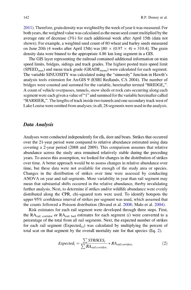
total scat on that segment by the overall mortality rate for that species (Eq. 2).
Expected i ¼
P
STRIKES i
P
RA rail corridor i
à RA rail corridor i
ð2Þ
142
B.P. Dorsey et al.
both years, the weighted value was calculated as the mean seed count multiplied by the
average rate of decrease (3%) for each additional week after April 15th (data not
shown). For example, a weighted seed count of 80 wheat and barley seeds measured
on June 20th (4 weeks after April 15th) was [80 Â (0.97 Â 4) = 310.4]. The grain
density data were binned to the appropriate 4.86 km long segment in a GIS.
The GIS layer representing the railroad contained additional information on train
speed limits, bridges, sidings and track grades. The highest posted train speed limit
(SPEED max ) and mean track grade (GRADE mean ) were calculated for each segment.
The variable SINUOSITY was calculated using the “sinuosity” function in Hawth’s
analysis tools extension for ArcGIS 9 (ESRI Redlands, CA 2004). The number of
bridges were counted and summed for the variable, hereinafter termed “BRIDGE c ”.
A count of vehicle overpasses, tunnels, snow sheds or rock cuts occurring along each
segment were each given a value of “1” and summed for the variable hereinafter called
“BARRIER c ”. The lengths of track inside two tunnels and one secondary track west of
Lake Louise were omitted from analyses; in all, 28 segments were used in the analysis.
Data Analysis
Analyses were conducted independently for elk, deer and bears. Strikes that occurred
over the 21-year period were compared to relative abundance estimated using data
covering a 2-year period (2008 and 2009). This comparison assumes that relative
abundance across the study area remained relatively stable during the preceding
years. To assess this assumption, we looked for changes in the distribution of strikes
over time. A better approach would be to assess changes in relative abundance over
time, but these data were not available for enough of the study area or species.
Changes in the distribution of strikes over time were assessed by conducting
ANOVA on year and rail segments. More variability in year than rail segment may
mean that substantial shifts occurred in the relative abundance, therby invalidating
further analysis. Next, to determine if strikes and/or wildlife abundance were evenly
distributed along the CPR, chi-squared tests were used. To identify hotspots the
upper 95% confidence interval of strikes per segment was used, which assumed that
the counts followed a Poisson distribution (Bivand et al. 2008; Malo et al. 2004).
Risk estimates for each rail segment were developed through three steps. First,
the RA rail corridor or RA rail bed estimates for each segment (i) were converted to a
percentage of the total from all rail segments. Next, the expected number of strikes
for each rail segment (Expected (i) ) was calculated by multiplying the percent of
total scat on that segment by the overall mortality rate for that species (Eq. 2).
Expected i ¼
P
STRIKES i
P
RA rail corridor i
à RA rail corridor i
ð2Þ
142
B.P. Dorsey et al.