

50
4 Design Optimization of Micromixers
may pick a solution on the Pareto-optimal front depending on his/her needs. Afzal
and Kim [31] used mixing effectiveness to pick an optimum design among available
Pareto-optimal solutions.
4.2 Conventional Versus Surrogate-Based Optimization
Various approaches have been used by researchers for optimization of a typical
system characterized by a set of inputs and responses. The most basic approach is
parametric study, which involves studying the effects of each design parameter on
system responses, keeping other parameters fixed. A more advanced approach is the
use of design of experiment (DOE) techniques. In DOE procedures, multiple parameters can be manipulated determining their effects on system response. Examples of
DOE are factorial designs, Latin hypercube sampling, etc.
Using the above mentioned approaches, it is possible to find acceptable or workable designs. Nonetheless, the urge to find the optimum design remains the most
important part. Therefore, optimization can be performed to search the entire design
space using a suitable optimization algorithm to maximize or minimize a system
response. It can be achieved using either gradient–based methods for constrained and
unconstrained optimization, or heuristic techniques like particle swarm optimization.
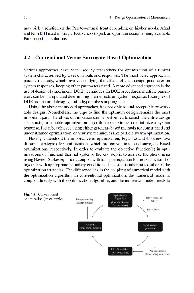
Having understood the importance of optimization, Figs. 4.5 and 4.6 show two
different strategies for optimization, which are conventional and surrogate-based
optimizations, respectively. In order to evaluate the objective function(s) in optimizations of fluid and thermal systems, the key step is to analyze the phenomena
using Navier–Stokes equations coupled with transport equation for heat/mass transfer
together with appropriate boundary conditions. This step is inherent to either of the
optimization strategies. The difference lies in the coupling of numerical model with
the optimization algorithm. In conventional optimization, the numerical model is
coupled directly with the optimization algorithm, and the numerical model needs to
Fig. 4.5 Conventional
optimization (an example)
4 Design Optimization of Micromixers
may pick a solution on the Pareto-optimal front depending on his/her needs. Afzal
and Kim [31] used mixing effectiveness to pick an optimum design among available
Pareto-optimal solutions.
4.2 Conventional Versus Surrogate-Based Optimization
Various approaches have been used by researchers for optimization of a typical
system characterized by a set of inputs and responses. The most basic approach is
parametric study, which involves studying the effects of each design parameter on
system responses, keeping other parameters fixed. A more advanced approach is the
use of design of experiment (DOE) techniques. In DOE procedures, multiple parameters can be manipulated determining their effects on system response. Examples of
DOE are factorial designs, Latin hypercube sampling, etc.
Using the above mentioned approaches, it is possible to find acceptable or workable designs. Nonetheless, the urge to find the optimum design remains the most
important part. Therefore, optimization can be performed to search the entire design
space using a suitable optimization algorithm to maximize or minimize a system
response. It can be achieved using either gradient–based methods for constrained and
unconstrained optimization, or heuristic techniques like particle swarm optimization.
Having understood the importance of optimization, Figs. 4.5 and 4.6 show two
different strategies for optimization, which are conventional and surrogate-based
optimizations, respectively. In order to evaluate the objective function(s) in optimizations of fluid and thermal systems, the key step is to analyze the phenomena
using Navier–Stokes equations coupled with transport equation for heat/mass transfer
together with appropriate boundary conditions. This step is inherent to either of the
optimization strategies. The difference lies in the coupling of numerical model with
the optimization algorithm. In conventional optimization, the numerical model is
coupled directly with the optimization algorithm, and the numerical model needs to
Fig. 4.5 Conventional
optimization (an example)