

3.1 Eulerian Approach to Mixing
37
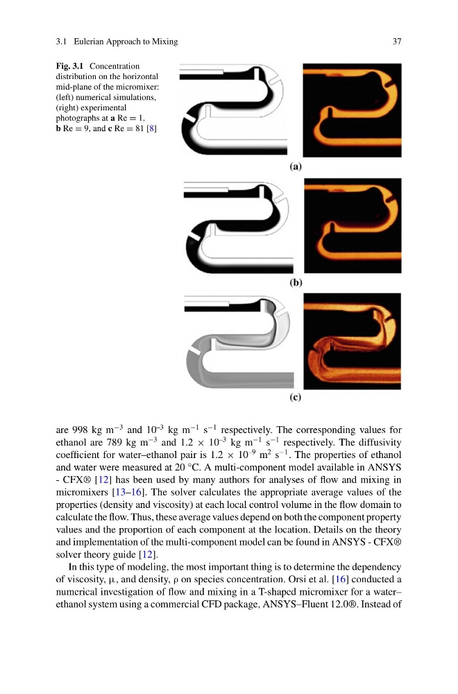
Fig. 3.1 Concentration
distribution on the horizontal
mid-plane of the micromixer:
(left) numerical simulations,
(right) experimental
photographs at a Re = 1,
b Re = 9, and c Re = 81 [8]
are 998 kg m
−3 and 10
–3 kg m
−1 s
−1 respectively. The corresponding values for
ethanol are 789 kg m
−3 and 1.2 × 10
–3 kg m
−1 s
−1 respectively. The diffusivity
coefficient for water–ethanol pair is 1.2 × 10
–9 m
2 s
−1 . The properties of ethanol
and water were measured at 20 °C. A multi-component model available in ANSYS
- CFX® [12] has been used by many authors for analyses of flow and mixing in
micromixers [13–16]. The solver calculates the appropriate average values of the
properties (density and viscosity) at each local control volume in the flow domain to
calculate the flow. Thus, these average values depend on both the component property
values and the proportion of each component at the location. Details on the theory
and implementation of the multi-component model can be found in ANSYS - CFX®
solver theory guide [12].
In this type of modeling, the most important thing is to determine the dependency
of viscosity, μ, and density, ρ on species concentration. Orsi et al. [16] conducted a
numerical investigation of flow and mixing in a T-shaped micromixer for a water–
ethanol system using a commercial CFD package, ANSYS–Fluent 12.0®. Instead of
37
Fig. 3.1 Concentration
distribution on the horizontal
mid-plane of the micromixer:
(left) numerical simulations,
(right) experimental
photographs at a Re = 1,
b Re = 9, and c Re = 81 [8]
are 998 kg m
−3 and 10
–3 kg m
−1 s
−1 respectively. The corresponding values for
ethanol are 789 kg m
−3 and 1.2 × 10
–3 kg m
−1 s
−1 respectively. The diffusivity
coefficient for water–ethanol pair is 1.2 × 10
–9 m
2 s
−1 . The properties of ethanol
and water were measured at 20 °C. A multi-component model available in ANSYS
- CFX® [12] has been used by many authors for analyses of flow and mixing in
micromixers [13–16]. The solver calculates the appropriate average values of the
properties (density and viscosity) at each local control volume in the flow domain to
calculate the flow. Thus, these average values depend on both the component property
values and the proportion of each component at the location. Details on the theory
and implementation of the multi-component model can be found in ANSYS - CFX®
solver theory guide [12].
In this type of modeling, the most important thing is to determine the dependency
of viscosity, μ, and density, ρ on species concentration. Orsi et al. [16] conducted a
numerical investigation of flow and mixing in a T-shaped micromixer for a water–
ethanol system using a commercial CFD package, ANSYS–Fluent 12.0®. Instead of