

36
3 Computational Analysis of Flow and Mixing in Micromixers
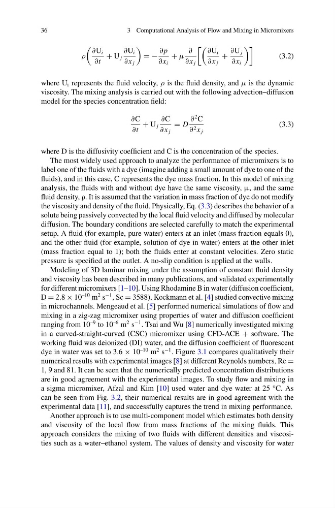
ρ
∂U i
∂t
+ U j
∂U i
∂ x j
= −
∂ p
∂ x i
+ μ
∂
∂ x j
∂U i
∂ x j
+
∂U j
∂ x i
(3.2)
where U i represents the fluid velocity, ρ is the fluid density, and μ is the dynamic
viscosity. The mixing analysis is carried out with the following advection–diffusion
model for the species concentration field:
∂C
∂t
+ U j
∂C
∂ x j
= D
∂
2 C
∂ 2 x j
(3.3)
where D is the diffusivity coefficient and C is the concentration of the species.
The most widely used approach to analyze the performance of micromixers is to
label one of the fluids with a dye (imagine adding a small amount of dye to one of the
fluids), and in this case, C represents the dye mass fraction. In this model of mixing
analysis, the fluids with and without dye have the same viscosity, μ, and the same
fluid density, ρ. It is assumed that the variation in mass fraction of dye do not modify
the viscosity and density of the fluid. Physically, Eq. (3.3) describes the behavior of a
solute being passively convected by the local fluid velocity and diffused by molecular
diffusion. The boundary conditions are selected carefully to match the experimental
setup. A fluid (for example, pure water) enters at an inlet (mass fraction equals 0),
and the other fluid (for example, solution of dye in water) enters at the other inlet
(mass fraction equal to 1); both the fluids enter at constant velocities. Zero static
pressure is specified at the outlet. A no-slip condition is applied at the walls.
Modeling of 3D laminar mixing under the assumption of constant fluid density
and viscosity has been described in many publications, and validated experimentally
for different micromixers [1–10]. Using Rhodamine B in water (diffusion coefficient,
D = 2.8 × 10
–10 m
2 s
−1 , Sc = 3588), Kockmann et al. [4] studied convective mixing
in microchannels. Mengeaud et al. [5] performed numerical simulations of flow and
mixing in a zig-zag micromixer using properties of water and diffusion coefficient
ranging from 10
–9 to 10
–6 m
2 s
−1 . Tsai and Wu [8] numerically investigated mixing
in a curved-straight-curved (CSC) micromixer using CFD-ACE + software. The
working fluid was deionized (DI) water, and the diffusion coefficient of fluorescent
dye in water was set to 3.6 × 10
–10 m
2 s
−1 . Figure 3.1 compares qualitatively their
numerical results with experimental images [8] at different Reynolds numbers, Re =
1, 9 and 81. It can be seen that the numerically predicted concentration distributions
are in good agreement with the experimental images. To study flow and mixing in
a sigma micromixer, Afzal and Kim [10] used water and dye water at 25 °C. As
can be seen from Fig. 3.2, their numerical results are in good agreement with the
experimental data [11], and successfully captures the trend in mixing performance.
Another approach is to use multi-component model which estimates both density
and viscosity of the local flow from mass fractions of the mixing fluids. This
approach considers the mixing of two fluids with different densities and viscosities such as a water–ethanol system. The values of density and viscosity for water
3 Computational Analysis of Flow and Mixing in Micromixers
ρ
∂U i
∂t
+ U j
∂U i
∂ x j
= −
∂ p
∂ x i
+ μ
∂
∂ x j
∂U i
∂ x j
+
∂U j
∂ x i
(3.2)
where U i represents the fluid velocity, ρ is the fluid density, and μ is the dynamic
viscosity. The mixing analysis is carried out with the following advection–diffusion
model for the species concentration field:
∂C
∂t
+ U j
∂C
∂ x j
= D
∂
2 C
∂ 2 x j
(3.3)
where D is the diffusivity coefficient and C is the concentration of the species.
The most widely used approach to analyze the performance of micromixers is to
label one of the fluids with a dye (imagine adding a small amount of dye to one of the
fluids), and in this case, C represents the dye mass fraction. In this model of mixing
analysis, the fluids with and without dye have the same viscosity, μ, and the same
fluid density, ρ. It is assumed that the variation in mass fraction of dye do not modify
the viscosity and density of the fluid. Physically, Eq. (3.3) describes the behavior of a
solute being passively convected by the local fluid velocity and diffused by molecular
diffusion. The boundary conditions are selected carefully to match the experimental
setup. A fluid (for example, pure water) enters at an inlet (mass fraction equals 0),
and the other fluid (for example, solution of dye in water) enters at the other inlet
(mass fraction equal to 1); both the fluids enter at constant velocities. Zero static
pressure is specified at the outlet. A no-slip condition is applied at the walls.
Modeling of 3D laminar mixing under the assumption of constant fluid density
and viscosity has been described in many publications, and validated experimentally
for different micromixers [1–10]. Using Rhodamine B in water (diffusion coefficient,
D = 2.8 × 10
–10 m
2 s
−1 , Sc = 3588), Kockmann et al. [4] studied convective mixing
in microchannels. Mengeaud et al. [5] performed numerical simulations of flow and
mixing in a zig-zag micromixer using properties of water and diffusion coefficient
ranging from 10
–9 to 10
–6 m
2 s
−1 . Tsai and Wu [8] numerically investigated mixing
in a curved-straight-curved (CSC) micromixer using CFD-ACE + software. The
working fluid was deionized (DI) water, and the diffusion coefficient of fluorescent
dye in water was set to 3.6 × 10
–10 m
2 s
−1 . Figure 3.1 compares qualitatively their
numerical results with experimental images [8] at different Reynolds numbers, Re =
1, 9 and 81. It can be seen that the numerically predicted concentration distributions
are in good agreement with the experimental images. To study flow and mixing in
a sigma micromixer, Afzal and Kim [10] used water and dye water at 25 °C. As
can be seen from Fig. 3.2, their numerical results are in good agreement with the
experimental data [11], and successfully captures the trend in mixing performance.
Another approach is to use multi-component model which estimates both density
and viscosity of the local flow from mass fractions of the mixing fluids. This
approach considers the mixing of two fluids with different densities and viscosities such as a water–ethanol system. The values of density and viscosity for water