

3.4 Monte Carlo Simulations
29
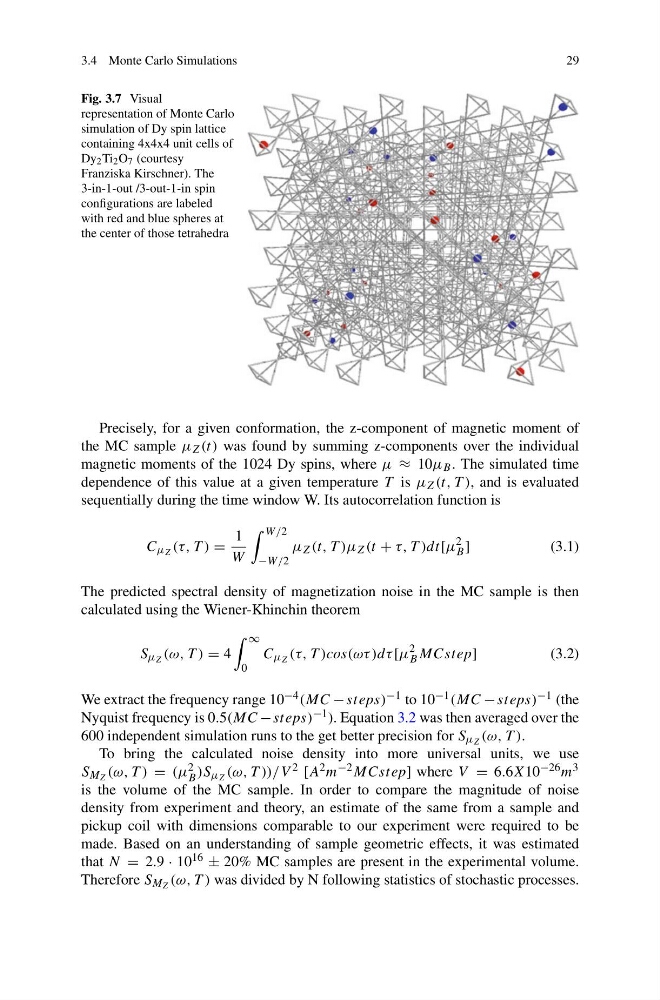
Fig. 3.7 Visual
representation of Monte Carlo
simulation of Dy spin lattice
containing 4x4x4 unit cells of
Dy 2 Ti 2 O 7 (courtesy
Franziska Kirschner). The
3-in-1-out /3-out-1-in spin
configurations are labeled
with red and blue spheres at
the center of those tetrahedra
Precisely, for a given conformation, the z-component of magnetic moment of
the MC sample μ Z (t) was found by summing z-components over the individual
magnetic moments of the 1024 Dy spins, where μ ≈ 10μ B . The simulated time
dependence of this value at a given temperature T is μ Z (t, T ), and is evaluated
sequentially during the time window W. Its autocorrelation function is
C μ Z (τ, T ) =
1
W
W/2
−W/2
μ Z (t, T )μ Z (t + τ, T )dt[μ
2
B ]
(3.1)
The predicted spectral density of magnetization noise in the MC sample is then
calculated using the Wiener-Khinchin theorem
S μ Z (ω, T ) = 4
∞
0
C μ Z (τ, T )cos(ωτ )dτ [μ
2
B MCstep]
(3.2)
We extract the frequency range 10 −4 (MC − steps) −1 to 10 −1 (MC − steps) −1 (the
Nyquist frequency is 0.5(MC − steps) −1 ). Equation 3.2 was then averaged over the
600 independent simulation runs to the get better precision for S μ Z (ω, T ).
To bring the calculated noise density into more universal units, we use
S M Z (ω, T ) = (μ 2
B )S μ Z (ω, T ))/V 2 [A 2 m −2 MCstep] where V = 6.6X10 −26 m 3
is the volume of the MC sample. In order to compare the magnitude of noise
density from experiment and theory, an estimate of the same from a sample and
pickup coil with dimensions comparable to our experiment were required to be
made. Based on an understanding of sample geometric effects, it was estimated
that N = 2.9 · 10 16 ± 20% MC samples are present in the experimental volume.
Therefore S M Z (ω, T ) was divided by N following statistics of stochastic processes.
29
Fig. 3.7 Visual
representation of Monte Carlo
simulation of Dy spin lattice
containing 4x4x4 unit cells of
Dy 2 Ti 2 O 7 (courtesy
Franziska Kirschner). The
3-in-1-out /3-out-1-in spin
configurations are labeled
with red and blue spheres at
the center of those tetrahedra
Precisely, for a given conformation, the z-component of magnetic moment of
the MC sample μ Z (t) was found by summing z-components over the individual
magnetic moments of the 1024 Dy spins, where μ ≈ 10μ B . The simulated time
dependence of this value at a given temperature T is μ Z (t, T ), and is evaluated
sequentially during the time window W. Its autocorrelation function is
C μ Z (τ, T ) =
1
W
W/2
−W/2
μ Z (t, T )μ Z (t + τ, T )dt[μ
2
B ]
(3.1)
The predicted spectral density of magnetization noise in the MC sample is then
calculated using the Wiener-Khinchin theorem
S μ Z (ω, T ) = 4
∞
0
C μ Z (τ, T )cos(ωτ )dτ [μ
2
B MCstep]
(3.2)
We extract the frequency range 10 −4 (MC − steps) −1 to 10 −1 (MC − steps) −1 (the
Nyquist frequency is 0.5(MC − steps) −1 ). Equation 3.2 was then averaged over the
600 independent simulation runs to the get better precision for S μ Z (ω, T ).
To bring the calculated noise density into more universal units, we use
S M Z (ω, T ) = (μ 2
B )S μ Z (ω, T ))/V 2 [A 2 m −2 MCstep] where V = 6.6X10 −26 m 3
is the volume of the MC sample. In order to compare the magnitude of noise
density from experiment and theory, an estimate of the same from a sample and
pickup coil with dimensions comparable to our experiment were required to be
made. Based on an understanding of sample geometric effects, it was estimated
that N = 2.9 · 10 16 ± 20% MC samples are present in the experimental volume.
Therefore S M Z (ω, T ) was divided by N following statistics of stochastic processes.