

28
3 Experiment
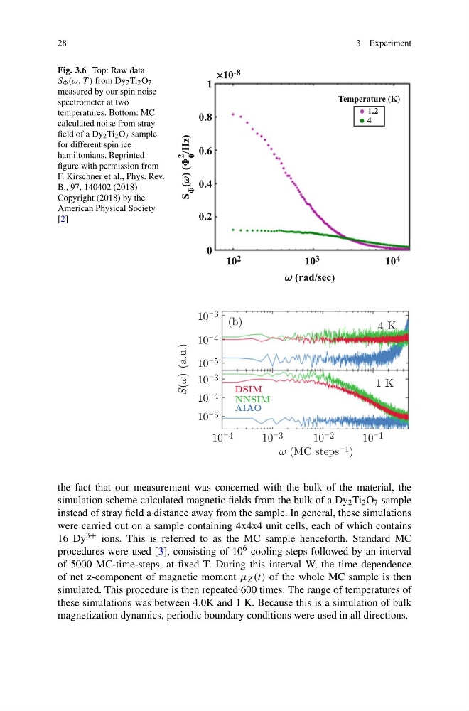
Fig. 3.6 Top: Raw data
S (ω, T ) from Dy 2 Ti 2 O 7
measured by our spin noise
spectrometer at two
temperatures. Bottom: MC
calculated noise from stray
field of a Dy 2 Ti 2 O 7 sample
for different spin ice
hamiltonians. Reprinted
figure with permission from
F. Kirschner et al., Phys. Rev.
B., 97, 140402 (2018)
Copyright (2018) by the
American Physical Society
[2]
1
Temperature (K)
0.8
0.6
0.4
0.2
0
¥10 -8
10 2
10 3
10 4
1.2
4
(rad/sec)
S ( ) (
0
2
/Hz)
10¯ 3 (b)
DSIM
NNSIM
AIAO
10¯ 4
10¯ 5
10¯ 3
10¯ 4
10¯ 5
4 K
1 K
10¯ 4
10¯ 3
10¯ 2
10¯ 1
S(ω) (a.u.)
ω (MC steps¯ 1 )
the fact that our measurement was concerned with the bulk of the material, the
simulation scheme calculated magnetic fields from the bulk of a Dy 2 Ti 2 O 7 sample
instead of stray field a distance away from the sample. In general, these simulations
were carried out on a sample containing 4x4x4 unit cells, each of which contains
16 Dy 3+ ions. This is referred to as the MC sample henceforth. Standard MC
procedures were used [3], consisting of 10 6 cooling steps followed by an interval
of 5000 MC-time-steps, at fixed T. During this interval W, the time dependence
of net z-component of magnetic moment μ Z (t) of the whole MC sample is then
simulated. This procedure is then repeated 600 times. The range of temperatures of
these simulations was between 4.0K and 1 K. Because this is a simulation of bulk
magnetization dynamics, periodic boundary conditions were used in all directions.
3 Experiment
Fig. 3.6 Top: Raw data
S (ω, T ) from Dy 2 Ti 2 O 7
measured by our spin noise
spectrometer at two
temperatures. Bottom: MC
calculated noise from stray
field of a Dy 2 Ti 2 O 7 sample
for different spin ice
hamiltonians. Reprinted
figure with permission from
F. Kirschner et al., Phys. Rev.
B., 97, 140402 (2018)
Copyright (2018) by the
American Physical Society
[2]
1
Temperature (K)
0.8
0.6
0.4
0.2
0
¥10 -8
10 2
10 3
10 4
1.2
4
(rad/sec)
S ( ) (
0
2
/Hz)
10¯ 3 (b)
DSIM
NNSIM
AIAO
10¯ 4
10¯ 5
10¯ 3
10¯ 4
10¯ 5
4 K
1 K
10¯ 4
10¯ 3
10¯ 2
10¯ 1
S(ω) (a.u.)
ω (MC steps¯ 1 )
the fact that our measurement was concerned with the bulk of the material, the
simulation scheme calculated magnetic fields from the bulk of a Dy 2 Ti 2 O 7 sample
instead of stray field a distance away from the sample. In general, these simulations
were carried out on a sample containing 4x4x4 unit cells, each of which contains
16 Dy 3+ ions. This is referred to as the MC sample henceforth. Standard MC
procedures were used [3], consisting of 10 6 cooling steps followed by an interval
of 5000 MC-time-steps, at fixed T. During this interval W, the time dependence
of net z-component of magnetic moment μ Z (t) of the whole MC sample is then
simulated. This procedure is then repeated 600 times. The range of temperatures of
these simulations was between 4.0K and 1 K. Because this is a simulation of bulk
magnetization dynamics, periodic boundary conditions were used in all directions.