

2 Principal Physics of Radar Location and Radio-Navigation
9
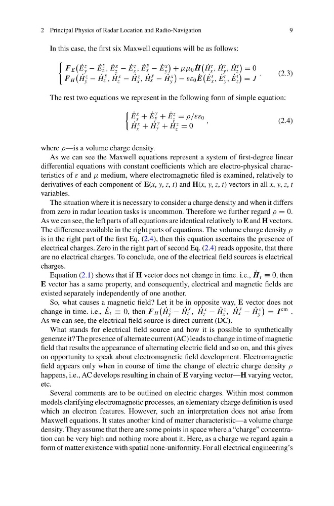
In this case, the first six Maxwell equations will be as follows:
F E
˙
E
z
y − ˙
E
y
z , ˙
E
x
z − ˙
E
z
x , ˙
E
y
x − ˙
E
x
y
+ μμ 0 ˙
H
˙
H
t
x , ˙
H
t
y , ˙
H
t
z
= 0
F H
˙
H
z
y − ˙
H
y
z , ˙
H
x
z − ˙
H
z
x , ˙
H
y
x − ˙
H
x
y
− εε 0 ˙
E
˙
E
t
x , ˙
E
t
y , ˙
E
t
z
= J
.
(2.3)
The rest two equations we represent in the following form of simple equation:
˙
E
x
x + ˙
E
y
y + ˙
E
z
z = ρ/εε 0
˙
H
x
x + ˙
H
y
y + ˙
H
z
z = 0
,
(2.4)
where ρ—is a volume charge density.
As we can see the Maxwell equations represent a system of first-degree linear
differential equations with constant coefficients which are electro-physical characteristics of ε and μ medium, where electromagnetic filed is examined, relatively to
derivatives of each component of E(x, y, z, t) and H(x, y, z, t) vectors in all x, y, z, t
variables.
The situation where it is necessary to consider a charge density and when it differs
from zero in radar location tasks is uncommon. Therefore we further regard ρ = 0.
As we can see, the left parts of all equations are identical relatively to E and H vectors.
The difference available in the right parts of equations. The volume charge density ρ
is in the right part of the first Eq. (2.4), then this equation ascertains the presence of
electrical charges. Zero in the right part of second Eq. (2.4) reads opposite, that there
are no electrical charges. To conclude, one of the electrical field sources is electrical
charges.
Equation (2.1) shows that if H vector does not change in time. i.e., ˙
H t ≡ 0, then
E vector has a same property, and consequently, electrical and magnetic fields are
existed separately independently of one another.
So, what causes a magnetic field? Let it be in opposite way, E vector does not
change in time. i.e., ˙
E t ≡ 0, then F H
˙
H
z
y − ˙
H
y
z , ˙
H
x
z − ˙
H
z
x , ˙
H
y
x − ˙
H
x
y
= I
cm .
As we can see, the electrical field source is direct current (DC).
What stands for electrical field source and how it is possible to synthetically
generate it? The presence of alternate current (AC) leads to change in time of magnetic
field that results the appearance of alternating electric field and so on, and this gives
on opportunity to speak about electromagnetic field development. Electromagnetic
field appears only when in course of time the change of electric charge density ρ
happens, i.e., AC develops resulting in chain of E varying vector—H varying vector,
etc.
Several comments are to be outlined on electric charges. Within most common
models clarifying electromagnetic processes, an elementary charge definition is used
which an electron features. However, such an interpretation does not arise from
Maxwell equations. It states another kind of matter characteristic—a volume charge
density. They assume that there are some points in space where a “charge” concentration can be very high and nothing more about it. Here, as a charge we regard again a
form of matter existence with spatial none-uniformity. For all electrical engineering’s
9
In this case, the first six Maxwell equations will be as follows:
F E
˙
E
z
y − ˙
E
y
z , ˙
E
x
z − ˙
E
z
x , ˙
E
y
x − ˙
E
x
y
+ μμ 0 ˙
H
˙
H
t
x , ˙
H
t
y , ˙
H
t
z
= 0
F H
˙
H
z
y − ˙
H
y
z , ˙
H
x
z − ˙
H
z
x , ˙
H
y
x − ˙
H
x
y
− εε 0 ˙
E
˙
E
t
x , ˙
E
t
y , ˙
E
t
z
= J
.
(2.3)
The rest two equations we represent in the following form of simple equation:
˙
E
x
x + ˙
E
y
y + ˙
E
z
z = ρ/εε 0
˙
H
x
x + ˙
H
y
y + ˙
H
z
z = 0
,
(2.4)
where ρ—is a volume charge density.
As we can see the Maxwell equations represent a system of first-degree linear
differential equations with constant coefficients which are electro-physical characteristics of ε and μ medium, where electromagnetic filed is examined, relatively to
derivatives of each component of E(x, y, z, t) and H(x, y, z, t) vectors in all x, y, z, t
variables.
The situation where it is necessary to consider a charge density and when it differs
from zero in radar location tasks is uncommon. Therefore we further regard ρ = 0.
As we can see, the left parts of all equations are identical relatively to E and H vectors.
The difference available in the right parts of equations. The volume charge density ρ
is in the right part of the first Eq. (2.4), then this equation ascertains the presence of
electrical charges. Zero in the right part of second Eq. (2.4) reads opposite, that there
are no electrical charges. To conclude, one of the electrical field sources is electrical
charges.
Equation (2.1) shows that if H vector does not change in time. i.e., ˙
H t ≡ 0, then
E vector has a same property, and consequently, electrical and magnetic fields are
existed separately independently of one another.
So, what causes a magnetic field? Let it be in opposite way, E vector does not
change in time. i.e., ˙
E t ≡ 0, then F H
˙
H
z
y − ˙
H
y
z , ˙
H
x
z − ˙
H
z
x , ˙
H
y
x − ˙
H
x
y
= I
cm .
As we can see, the electrical field source is direct current (DC).
What stands for electrical field source and how it is possible to synthetically
generate it? The presence of alternate current (AC) leads to change in time of magnetic
field that results the appearance of alternating electric field and so on, and this gives
on opportunity to speak about electromagnetic field development. Electromagnetic
field appears only when in course of time the change of electric charge density ρ
happens, i.e., AC develops resulting in chain of E varying vector—H varying vector,
etc.
Several comments are to be outlined on electric charges. Within most common
models clarifying electromagnetic processes, an elementary charge definition is used
which an electron features. However, such an interpretation does not arise from
Maxwell equations. It states another kind of matter characteristic—a volume charge
density. They assume that there are some points in space where a “charge” concentration can be very high and nothing more about it. Here, as a charge we regard again a
form of matter existence with spatial none-uniformity. For all electrical engineering’s