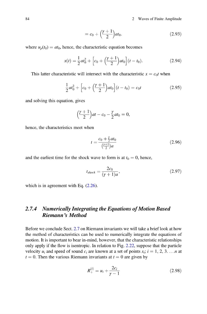
¼ c 0 þ
γ þ 1
2
at 0 :
ð2:93Þ
where u p (t 0 ) ¼ at 0 , hence, the characteristic equation becomes
x t
ð Þ ¼
1
2
at
2
0 þ c 0 þ
γ þ 1
2
at 0
h
i
t À t 0
ð
Þ:
ð2:94Þ
This latter characteristic will intersect with the characteristic x ¼ c 0 t when
1
2
at
2
0 þ c 0 þ
γ þ 1
2
at 0
h
i
t À t 0
ð
Þ¼c 0 t
ð2:95Þ
and solving this equation, gives
γ þ 1
2
at À c 0 À
γ
2
at 0 ¼ 0,
hence, the characteristics meet when
t ¼
c 0 þ
γ
2 at 0
γþ1
2
À Á
a
ð2:96Þ
and the earliest time for the shock wave to form is at t 0 ¼ 0, hence,
t shock ¼
2c 0
γ þ 1
ð
Þa
,
ð2:97Þ
which is in agreement with Eq. (2.26).
2.7.4 Numerically Integrating the Equations of Motion Based
Riemann’s Method
Before we conclude Sect. 2.7 on Riemann invariants we will take a brief look at how
the method of characteristics can be used to numerically integrate the equations of
motion. It is important to bear in-mind, however, that the characteristic relationships
only apply if the flow is isentropic. In relation to Fig. 2.22, suppose that the particle
velocity u i and speed of sound c i are known at a set of points x i ; i ¼ 1, 2, 3. . . .n at
t ¼ 0. Then the various Riemann invariants at t ¼ 0 are given by
R
i
ð Þ
þ ¼ u i þ
2c i
γ À 1
ð2:98Þ
84
2 Waves of Finite Amplitude