

and
R
i
ð Þ
À ¼ u i À
2c i
γ À 1
,
ð2:99Þ
where u i ¼ u(x i , 0) and c i ¼ c(x i , 0) for i ¼ 1, 2, 3. . . .n and all Riemann invariants are
known at t ¼ 0.
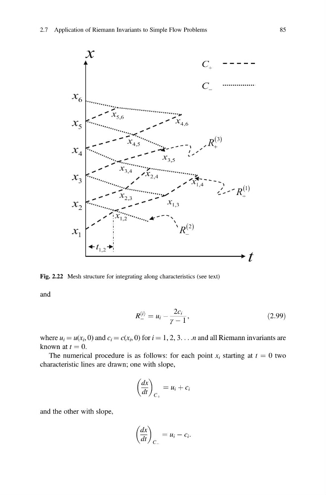
The numerical procedure is as follows: for each point x i starting at t ¼ 0 two
characteristic lines are drawn; one with slope,
dx
dt
C þ
¼ u i þ c i
and the other with slope,
dx
dt
C À
¼ u i À c i :
Fig. 2.22 Mesh structure for integrating along characteristics (see text)
2.7 Application of Riemann Invariants to Simple Flow Problems
85
R
i
ð Þ
À ¼ u i À
2c i
γ À 1
,
ð2:99Þ
where u i ¼ u(x i , 0) and c i ¼ c(x i , 0) for i ¼ 1, 2, 3. . . .n and all Riemann invariants are
known at t ¼ 0.
The numerical procedure is as follows: for each point x i starting at t ¼ 0 two
characteristic lines are drawn; one with slope,
dx
dt
C þ
¼ u i þ c i
and the other with slope,
dx
dt
C À
¼ u i À c i :
Fig. 2.22 Mesh structure for integrating along characteristics (see text)
2.7 Application of Riemann Invariants to Simple Flow Problems
85