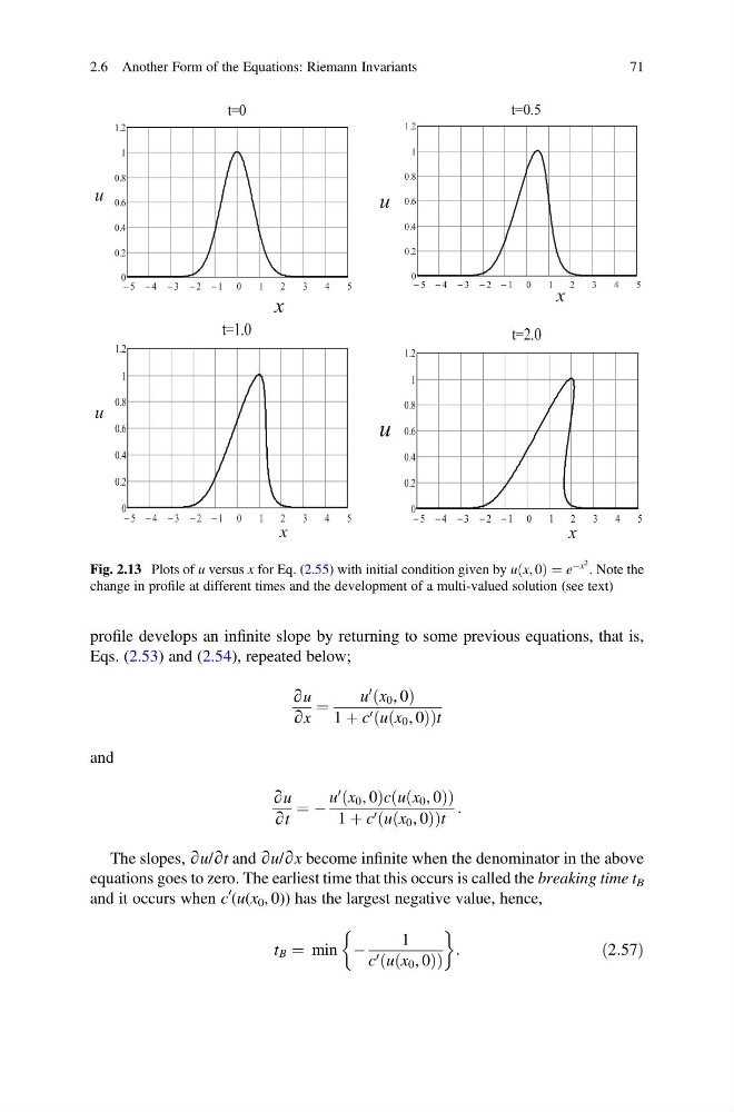
profile develops an infinite slope by returning to some previous equations, that is,
Eqs. (2.53) and (2.54), repeated below;
∂u
∂x
¼
u
0 x 0 , 0
ð
Þ
1 þ c 0 u x 0 , 0
ð
Þ
ð
Þ t
and
∂u
∂t
¼ À
u
0 x 0 , 0
ð
Þc u x 0 , 0
ð
Þ
ð
Þ
1 þ c 0 u x 0 , 0
ð
Þ
ð
Þ t
:
The slopes, ∂u/∂t and ∂u/∂x become infinite when the denominator in the above
equations goes to zero. The earliest time that this occurs is called the breaking time t B
and it occurs when c
0 (u(x 0 , 0)) has the largest negative value, hence,
t B ¼ min À
1
c 0 u x 0 , 0
ð
Þ
ð
Þ
&
'
:
ð2:57Þ
Fig. 2.13 Plots of u versus x for Eq. (2.55) with initial condition given by u x, 0
ð Þ ¼ e
Àx
2 . Note the
change in profile at different times and the development of a multi-valued solution (see text)
2.6 Another Form of the Equations: Riemann Invariants
71