

Therefore,
u x, t
ð Þ ¼ e
Àx
2
0 on the line t ¼ e
x
2
0 x À x 0
ð
Þ:
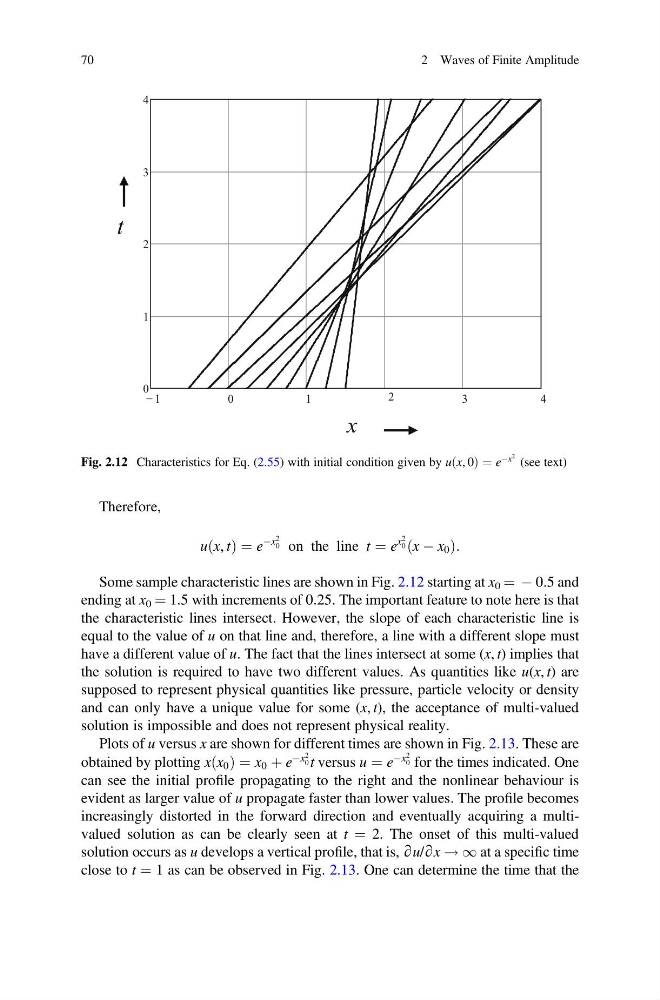
Some sample characteristic lines are shown in Fig. 2.12 starting at x 0 ¼ À 0.5 and
ending at x 0 ¼ 1.5 with increments of 0.25. The important feature to note here is that
the characteristic lines intersect. However, the slope of each characteristic line is
equal to the value of u on that line and, therefore, a line with a different slope must
have a different value of u. The fact that the lines intersect at some (x, t) implies that
the solution is required to have two different values. As quantities like u(x, t) are
supposed to represent physical quantities like pressure, particle velocity or density
and can only have a unique value for some (x, t), the acceptance of multi-valued
solution is impossible and does not represent physical reality.
Plots of u versus x are shown for different times are shown in Fig. 2.13. These are
obtained by plotting x x 0
ð Þ ¼ x 0 þ e
Àx
2
0 t versus u ¼ e
Àx
2
0 for the times indicated. One
can see the initial profile propagating to the right and the nonlinear behaviour is
evident as larger value of u propagate faster than lower values. The profile becomes
increasingly distorted in the forward direction and eventually acquiring a multivalued solution as can be clearly seen at t ¼ 2. The onset of this multi-valued
solution occurs as u develops a vertical profile, that is, ∂u/∂x ! 1 at a specific time
close to t ¼ 1 as can be observed in Fig. 2.13. One can determine the time that the
1
−
0
1
2
3
4
0
1
2
3
4
t
x
Fig. 2.12 Characteristics for Eq. (2.55) with initial condition given by u x, 0
ð Þ ¼ e
Àx
2 (see text)
70
2 Waves of Finite Amplitude
u x, t
ð Þ ¼ e
Àx
2
0 on the line t ¼ e
x
2
0 x À x 0
ð
Þ:
Some sample characteristic lines are shown in Fig. 2.12 starting at x 0 ¼ À 0.5 and
ending at x 0 ¼ 1.5 with increments of 0.25. The important feature to note here is that
the characteristic lines intersect. However, the slope of each characteristic line is
equal to the value of u on that line and, therefore, a line with a different slope must
have a different value of u. The fact that the lines intersect at some (x, t) implies that
the solution is required to have two different values. As quantities like u(x, t) are
supposed to represent physical quantities like pressure, particle velocity or density
and can only have a unique value for some (x, t), the acceptance of multi-valued
solution is impossible and does not represent physical reality.
Plots of u versus x are shown for different times are shown in Fig. 2.13. These are
obtained by plotting x x 0
ð Þ ¼ x 0 þ e
Àx
2
0 t versus u ¼ e
Àx
2
0 for the times indicated. One
can see the initial profile propagating to the right and the nonlinear behaviour is
evident as larger value of u propagate faster than lower values. The profile becomes
increasingly distorted in the forward direction and eventually acquiring a multivalued solution as can be clearly seen at t ¼ 2. The onset of this multi-valued
solution occurs as u develops a vertical profile, that is, ∂u/∂x ! 1 at a specific time
close to t ¼ 1 as can be observed in Fig. 2.13. One can determine the time that the
1
−
0
1
2
3
4
0
1
2
3
4
t
x
Fig. 2.12 Characteristics for Eq. (2.55) with initial condition given by u x, 0
ð Þ ¼ e
Àx
2 (see text)
70
2 Waves of Finite Amplitude