

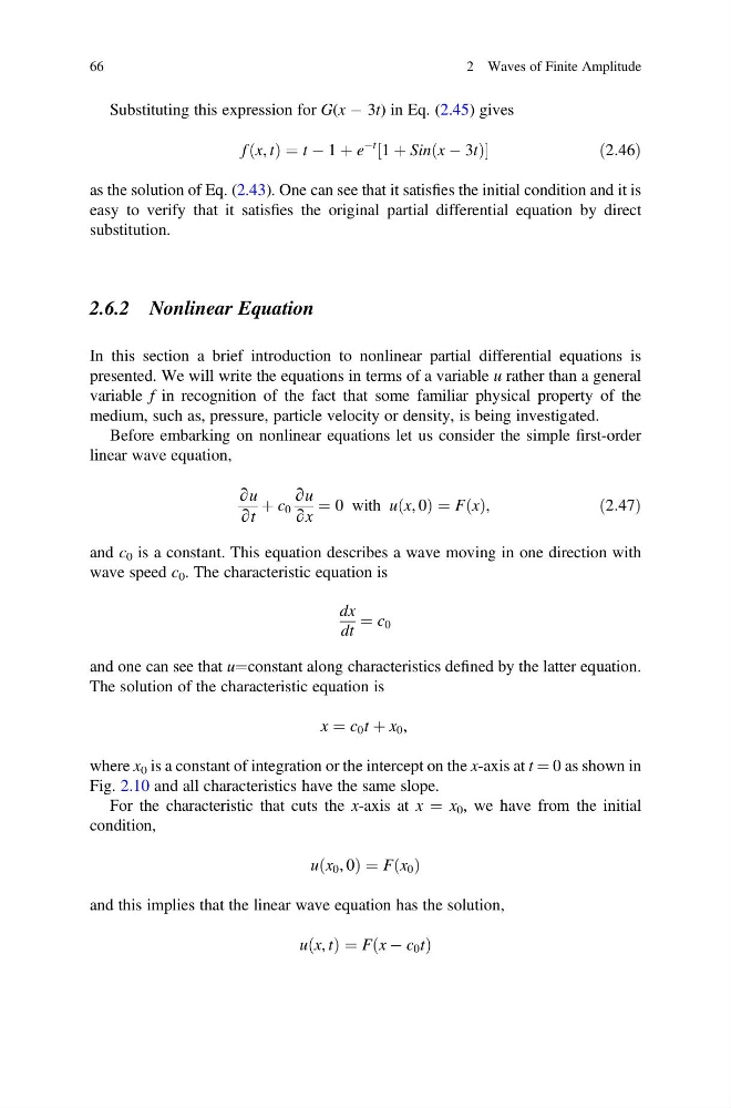
Substituting this expression for G(x À 3t) in Eq. (2.45) gives
f x, t
ð Þ ¼ t À 1 þ e
Àt 1 þ Sin x À 3t
ð
Þ
½
ð 2:46Þ
as the solution of Eq. (2.43). One can see that it satisfies the initial condition and it is
easy to verify that it satisfies the original partial differential equation by direct
substitution.
2.6.2 Nonlinear Equation
In this section a brief introduction to nonlinear partial differential equations is
presented. We will write the equations in terms of a variable u rather than a general
variable f in recognition of the fact that some familiar physical property of the
medium, such as, pressure, particle velocity or density, is being investigated.
Before embarking on nonlinear equations let us consider the simple first-order
linear wave equation,
∂u
∂t
þ c 0
∂u
∂x
¼ 0 with u x, 0
ð Þ ¼ F x
ð Þ,
ð2:47Þ
and c 0 is a constant. This equation describes a wave moving in one direction with
wave speed c 0 . The characteristic equation is
dx
dt
¼ c 0
and one can see that u¼constant along characteristics defined by the latter equation.
The solution of the characteristic equation is
x ¼ c 0 t þ x 0 ,
where x 0 is a constant of integration or the intercept on the x-axis at t ¼ 0 as shown in
Fig. 2.10 and all characteristics have the same slope.
For the characteristic that cuts the x-axis at x ¼ x 0 , we have from the initial
condition,
u x 0 , 0
ð
Þ ¼ F x 0
ð Þ
and this implies that the linear wave equation has the solution,
u x, t
ð Þ ¼ F x À c 0 t
ð
Þ
66
2 Waves of Finite Amplitude
f x, t
ð Þ ¼ t À 1 þ e
Àt 1 þ Sin x À 3t
ð
Þ
½
ð 2:46Þ
as the solution of Eq. (2.43). One can see that it satisfies the initial condition and it is
easy to verify that it satisfies the original partial differential equation by direct
substitution.
2.6.2 Nonlinear Equation
In this section a brief introduction to nonlinear partial differential equations is
presented. We will write the equations in terms of a variable u rather than a general
variable f in recognition of the fact that some familiar physical property of the
medium, such as, pressure, particle velocity or density, is being investigated.
Before embarking on nonlinear equations let us consider the simple first-order
linear wave equation,
∂u
∂t
þ c 0
∂u
∂x
¼ 0 with u x, 0
ð Þ ¼ F x
ð Þ,
ð2:47Þ
and c 0 is a constant. This equation describes a wave moving in one direction with
wave speed c 0 . The characteristic equation is
dx
dt
¼ c 0
and one can see that u¼constant along characteristics defined by the latter equation.
The solution of the characteristic equation is
x ¼ c 0 t þ x 0 ,
where x 0 is a constant of integration or the intercept on the x-axis at t ¼ 0 as shown in
Fig. 2.10 and all characteristics have the same slope.
For the characteristic that cuts the x-axis at x ¼ x 0 , we have from the initial
condition,
u x 0 , 0
ð
Þ ¼ F x 0
ð Þ
and this implies that the linear wave equation has the solution,
u x, t
ð Þ ¼ F x À c 0 t
ð
Þ
66
2 Waves of Finite Amplitude