

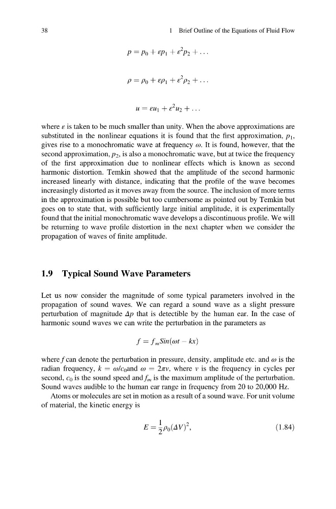
p ¼ p 0 þ εp 1 þ ε
2 p 2 þ . . .
ρ ¼ ρ 0 þ ερ 1 þ ε
2
ρ 2 þ . . .
u ¼ εu 1 þ ε
2 u 2 þ . . .
where ε is taken to be much smaller than unity. When the above approximations are
substituted in the nonlinear equations it is found that the first approximation, p 1 ,
gives rise to a monochromatic wave at frequency ω. It is found, however, that the
second approximation, p 2 , is also a monochromatic wave, but at twice the frequency
of the first approximation due to nonlinear effects which is known as second
harmonic distortion. Temkin showed that the amplitude of the second harmonic
increased linearly with distance, indicating that the profile of the wave becomes
increasingly distorted as it moves away from the source. The inclusion of more terms
in the approximation is possible but too cumbersome as pointed out by Temkin but
goes on to state that, with sufficiently large initial amplitude, it is experimentally
found that the initial monochromatic wave develops a discontinuous profile. We will
be returning to wave profile distortion in the next chapter when we consider the
propagation of waves of finite amplitude.
1.9 Typical Sound Wave Parameters
Let us now consider the magnitude of some typical parameters involved in the
propagation of sound waves. We can regard a sound wave as a slight pressure
perturbation of magnitude Δp that is detectible by the human ear. In the case of
harmonic sound waves we can write the perturbation in the parameters as
f ¼ f m Sin ωt À kx
ð
Þ
where f can denote the perturbation in pressure, density, amplitude etc. and ω is the
radian frequency, k ¼ ω/c 0 and ω ¼ 2πv, where v is the frequency in cycles per
second, c 0 is the sound speed and f m is the maximum amplitude of the perturbation.
Sound waves audible to the human ear range in frequency from 20 to 20,000 Hz.
Atoms or molecules are set in motion as a result of a sound wave. For unit volume
of material, the kinetic energy is
E ¼
1
2
ρ 0 ΔV
ð Þ
2 ,
ð1:84Þ
38
1 Brief Outline of the Equations of Fluid Flow
2 p 2 þ . . .
ρ ¼ ρ 0 þ ερ 1 þ ε
2
ρ 2 þ . . .
u ¼ εu 1 þ ε
2 u 2 þ . . .
where ε is taken to be much smaller than unity. When the above approximations are
substituted in the nonlinear equations it is found that the first approximation, p 1 ,
gives rise to a monochromatic wave at frequency ω. It is found, however, that the
second approximation, p 2 , is also a monochromatic wave, but at twice the frequency
of the first approximation due to nonlinear effects which is known as second
harmonic distortion. Temkin showed that the amplitude of the second harmonic
increased linearly with distance, indicating that the profile of the wave becomes
increasingly distorted as it moves away from the source. The inclusion of more terms
in the approximation is possible but too cumbersome as pointed out by Temkin but
goes on to state that, with sufficiently large initial amplitude, it is experimentally
found that the initial monochromatic wave develops a discontinuous profile. We will
be returning to wave profile distortion in the next chapter when we consider the
propagation of waves of finite amplitude.
1.9 Typical Sound Wave Parameters
Let us now consider the magnitude of some typical parameters involved in the
propagation of sound waves. We can regard a sound wave as a slight pressure
perturbation of magnitude Δp that is detectible by the human ear. In the case of
harmonic sound waves we can write the perturbation in the parameters as
f ¼ f m Sin ωt À kx
ð
Þ
where f can denote the perturbation in pressure, density, amplitude etc. and ω is the
radian frequency, k ¼ ω/c 0 and ω ¼ 2πv, where v is the frequency in cycles per
second, c 0 is the sound speed and f m is the maximum amplitude of the perturbation.
Sound waves audible to the human ear range in frequency from 20 to 20,000 Hz.
Atoms or molecules are set in motion as a result of a sound wave. For unit volume
of material, the kinetic energy is
E ¼
1
2
ρ 0 ΔV
ð Þ
2 ,
ð1:84Þ
38
1 Brief Outline of the Equations of Fluid Flow