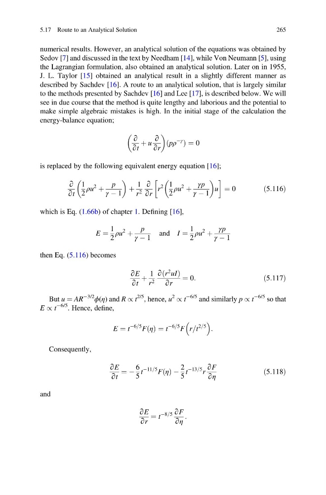
numerical results. However, an analytical solution of the equations was obtained by
Sedov [7] and discussed in the text by Needham [14], while Von Neumann [5], using
the Lagrangian formulation, also obtained an analytical solution. Later on in 1955,
J. L. Taylor [15] obtained an analytical result in a slightly different manner as
described by Sachdev [16]. A route to an analytical solution, that is largely similar
to the methods presented by Sachdev [16] and Lee [17], is described below. We will
see in due course that the method is quite lengthy and laborious and the potential to
make simple algebraic mistakes is high. In the initial stage of the calculation the
energy-balance equation;
∂
∂t
þ u
∂
∂r
pρ
Àγ
ð
Þ¼0
is replaced by the following equivalent energy equation [16];
∂
∂t
1
2
ρu
2
þ
p
γ À 1
þ
1
r 2
∂
∂r
r
2 1
2
ρu
2
þ
γp
γ À 1
u
!
¼ 0
ð5:116Þ
which is Eq. (1.66b) of chapter 1. Defining [16],
E ¼
1
2
ρu
2
þ
p
γ À 1
and I ¼
1
2
ρu
2
þ
γp
γ À 1
then Eq. (5.116) becomes
∂E
∂t
þ
1
r 2
∂ r
2 uI
ð
Þ
∂r
¼ 0:
ð5:117Þ
But u ¼ AR
À3/2
ϕ(η) and R / t
2/5
, hence, u
2
/ t
À6/5 and similarly p / t
À6/5 so that
E / t
À6/5 . Hence, define,
E ¼ t
À6=5 F η
ð Þ ¼ t
À6=5 F r=t
2=5
:
Consequently,
∂E
∂t
¼ À
6
5
t
À11=5 F η
ð Þ À
2
5
t
À13=5 r
∂F
∂η
ð5:118Þ
and
∂E
∂r
¼ t
À8=5 ∂F
∂η
:
5.17 Route to an Analytical Solution
265