

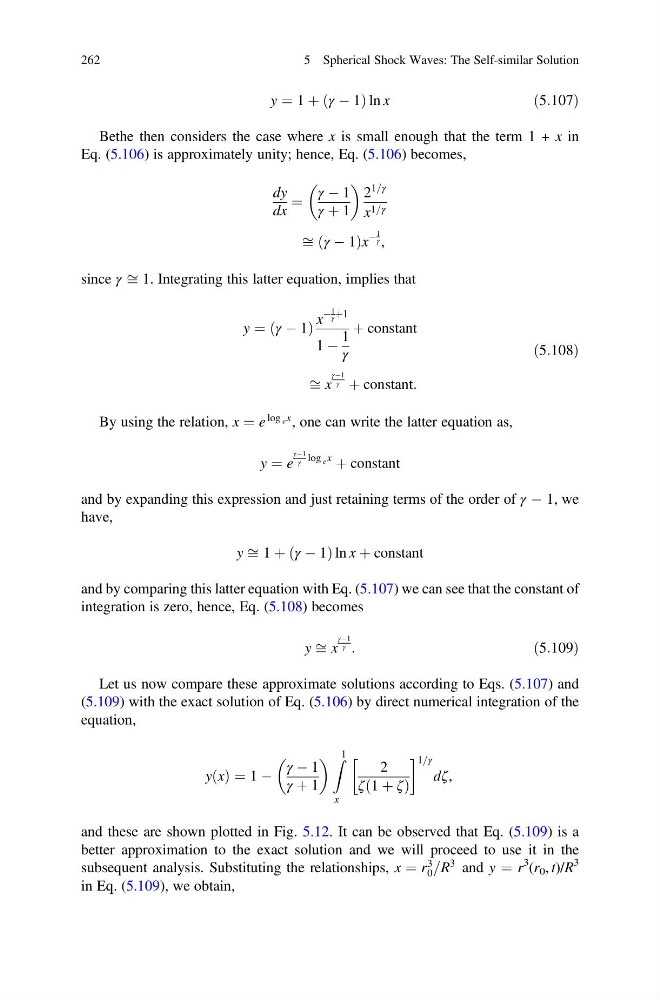
y ¼ 1 þ γ À 1
ð
Þln x
ð5:107Þ
Bethe then considers the case where x is small enough that the term 1 + x in
Eq. (5.106) is approximately unity; hence, Eq. (5.106) becomes,
dy
dx
¼
γ À 1
γ þ 1
2
1=γ
x 1=γ
ffi γ À 1
ð
Þx
À
1
γ ,
since γ ffi 1. Integrating this latter equation, implies that
y ¼ γ À 1
ð
Þ
x
À
1
γ þ1
1 À
1
γ
þ constant
ffi x
γÀ1
γ þ constant:
ð5:108Þ
By using the relation, x ¼ e
log e x , one can write the latter equation as,
y ¼ e
γÀ1
γ log e x
þ constant
and by expanding this expression and just retaining terms of the order of γ À 1, we
have,
y ffi 1 þ γ À 1
ð
Þln x þ constant
and by comparing this latter equation with Eq. (5.107) we can see that the constant of
integration is zero, hence, Eq. (5.108) becomes
y ffi x
γÀ1
γ :
ð5:109Þ
Let us now compare these approximate solutions according to Eqs. (5.107) and
(5.109) with the exact solution of Eq. (5.106) by direct numerical integration of the
equation,
y x
ð Þ ¼ 1 À
γ À 1
γ þ 1
Z 1
x
2
ζ 1 þ ζ
ð
Þ
! 1=γ
dζ,
and these are shown plotted in Fig. 5.12. It can be observed that Eq. (5.109) is a
better approximation to the exact solution and we will proceed to use it in the
subsequent analysis. Substituting the relationships, x ¼ r
3
0 =R
3 and y ¼ r
3 (r 0 , t)/R
3
in Eq. (5.109), we obtain,
262
5 Spherical Shock Waves: The Self-similar Solution
ð
Þln x
ð5:107Þ
Bethe then considers the case where x is small enough that the term 1 + x in
Eq. (5.106) is approximately unity; hence, Eq. (5.106) becomes,
dy
dx
¼
γ À 1
γ þ 1
2
1=γ
x 1=γ
ffi γ À 1
ð
Þx
À
1
γ ,
since γ ffi 1. Integrating this latter equation, implies that
y ¼ γ À 1
ð
Þ
x
À
1
γ þ1
1 À
1
γ
þ constant
ffi x
γÀ1
γ þ constant:
ð5:108Þ
By using the relation, x ¼ e
log e x , one can write the latter equation as,
y ¼ e
γÀ1
γ log e x
þ constant
and by expanding this expression and just retaining terms of the order of γ À 1, we
have,
y ffi 1 þ γ À 1
ð
Þln x þ constant
and by comparing this latter equation with Eq. (5.107) we can see that the constant of
integration is zero, hence, Eq. (5.108) becomes
y ffi x
γÀ1
γ :
ð5:109Þ
Let us now compare these approximate solutions according to Eqs. (5.107) and
(5.109) with the exact solution of Eq. (5.106) by direct numerical integration of the
equation,
y x
ð Þ ¼ 1 À
γ À 1
γ þ 1
Z 1
x
2
ζ 1 þ ζ
ð
Þ
! 1=γ
dζ,
and these are shown plotted in Fig. 5.12. It can be observed that Eq. (5.109) is a
better approximation to the exact solution and we will proceed to use it in the
subsequent analysis. Substituting the relationships, x ¼ r
3
0 =R
3 and y ¼ r
3 (r 0 , t)/R
3
in Eq. (5.109), we obtain,
262
5 Spherical Shock Waves: The Self-similar Solution