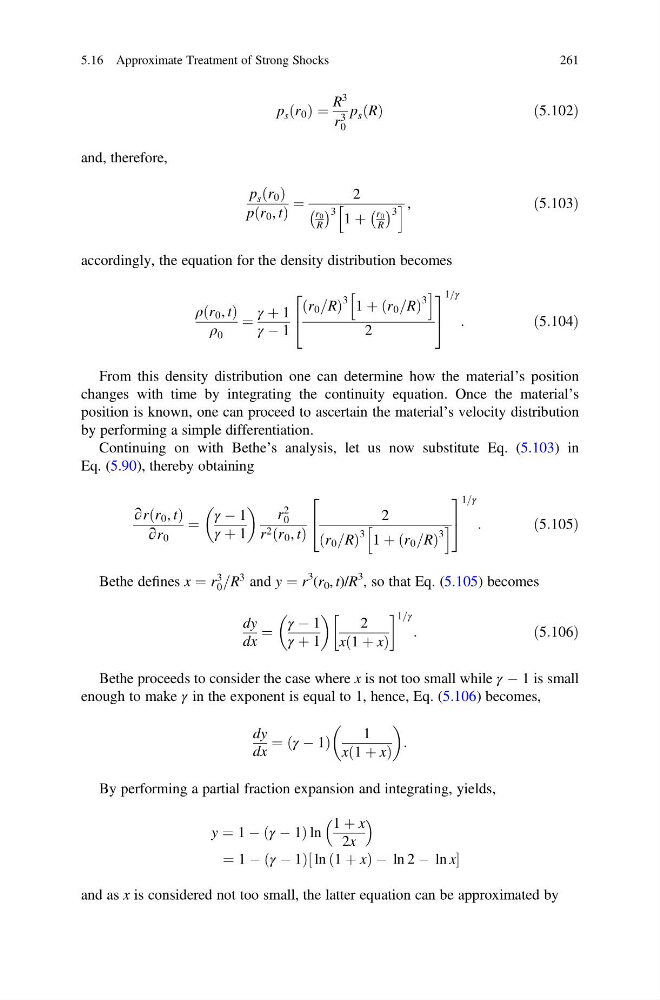
p s r 0
ð Þ ¼
R
3
r
3
0
p s R
ð Þ
ð5:102Þ
and, therefore,
p s r 0
ð Þ
p r 0 , t
ð
Þ
¼
2
r 0
R
À Á 3 1 þ
r 0
R
À Á 3
h
i,
ð5:103Þ
accordingly, the equation for the density distribution becomes
ρ r 0 , t
ð
Þ
ρ 0
¼
γ þ 1
γ À 1
r 0 =R
ð
Þ
3 1 þ r 0 =R
ð
Þ
3
h
i
2
2
4
3
5
1=γ
:
ð5:104Þ
From this density distribution one can determine how the material’s position
changes with time by integrating the continuity equation. Once the material’s
position is known, one can proceed to ascertain the material’s velocity distribution
by performing a simple differentiation.
Continuing on with Bethe’s analysis, let us now substitute Eq. (5.103) in
Eq. (5.90), thereby obtaining
∂r r 0 , t
ð
Þ
∂r 0
¼
γ À 1
γ þ 1
r
2
0
r 2 r 0 , t
ð
Þ
2
r 0 =R
ð
Þ
3 1 þ r 0 =R
ð
Þ
3
h
i
2
4
3
5
1=γ
:
ð5:105Þ
Bethe defines x ¼ r
3
0 =R
3 and y ¼ r
3 (r 0 , t)/R
3 , so that Eq. (5.105) becomes
dy
dx
¼
γ À 1
γ þ 1
2
x 1 þ x
ð
Þ
! 1=γ
:
ð5:106Þ
Bethe proceeds to consider the case where x is not too small while γ À 1 is small
enough to make γ in the exponent is equal to 1, hence, Eq. (5.106) becomes,
dy
dx
¼ γ À 1
ð
Þ
1
x 1 þ x
ð
Þ
:
By performing a partial fraction expansion and integrating, yields,
y ¼ 1 À γ À 1
ð
Þln
1 þ x
2x
¼ 1 À γ À 1
ð
Þ ln 1 þ x
ð
ÞÀ ln 2 À ln x
½
Š
and as x is considered not too small, the latter equation can be approximated by
5.16 Approximate Treatment of Strong Shocks
261