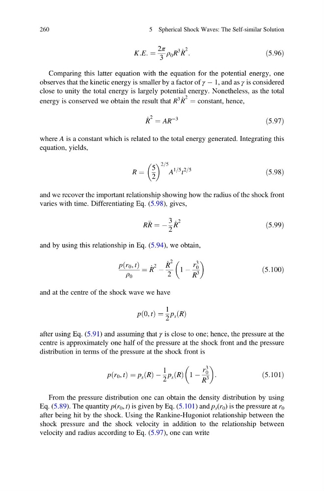
K:E: ¼
2π
3
ρ 0 R
3 _
R
2 :
ð5:96Þ
Comparing this latter equation with the equation for the potential energy, one
observes that the kinetic energy is smaller by a factor of γ À 1, and as γ is considered
close to unity the total energy is largely potential energy. Nonetheless, as the total
energy is conserved we obtain the result that R
3 _
R
2 ¼ constant, hence,
_
R
2 ¼ AR
À3
ð5:97Þ
where A is a constant which is related to the total energy generated. Integrating this
equation, yields,
R ¼
5
2
2=5
A
1=5 t
2=5
ð5:98Þ
and we recover the important relationship showing how the radius of the shock front
varies with time. Differentiating Eq. (5.98), gives,
R €
R ¼ À
3
2
_
R
2
ð5:99Þ
and by using this relationship in Eq. (5.94), we obtain,
p r 0 , t
ð
Þ
ρ 0
¼ _
R
2 À
_
R
2
2
1 À
r
3
0
R
3
ð5:100Þ
and at the centre of the shock wave we have
p 0, t
ð Þ ¼
1
2
p s R
ð Þ
after using Eq. (5.91) and assuming that γ is close to one; hence, the pressure at the
centre is approximately one half of the pressure at the shock front and the pressure
distribution in terms of the pressure at the shock front is
p r 0 , t
ð
Þ ¼ p s R
ð Þ À
1
2
p s R
ð Þ 1 À
r
3
0
R
3
:
ð5:101Þ
From the pressure distribution one can obtain the density distribution by using
Eq. (5.89). The quantity p(r 0 , t) is given by Eq. (5.101) and p s (r 0 ) is the pressure at r 0
after being hit by the shock. Using the Rankine-Hugoniot relationship between the
shock pressure and the shock velocity in addition to the relationship between
velocity and radius according to Eq. (5.97), one can write
260
5 Spherical Shock Waves: The Self-similar Solution