

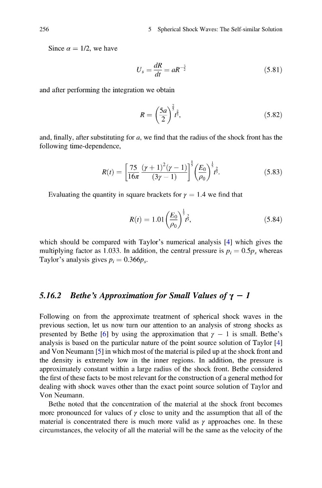
Since α ¼ 1/2, we have
U s ¼
dR
dt
¼ aR
À
3
2
ð5:81Þ
and after performing the integration we obtain
R ¼
5a
2
2
5
t
2
5 ,
ð5:82Þ
and, finally, after substituting for a, we find that the radius of the shock front has the
following time-dependence,
R t
ð Þ ¼
75
16π
γ þ 1
ð
Þ
2 γ À 1
ð
Þ
3γ À 1
ð
Þ
! 1
5
E 0
ρ 0
1
5
t
2
5 :
ð5:83Þ
Evaluating the quantity in square brackets for γ ¼ 1.4 we find that
R t
ð Þ ¼ 1:01
E 0
ρ 0
1
5
t
2
5 ,
ð5:84Þ
which should be compared with Taylor’s numerical analysis [4] which gives the
multiplying factor as 1.033. In addition, the central pressure is p i ¼ 0.5p s whereas
Taylor’s analysis gives p i ¼ 0.366p s .
5.16.2 Bethe’s Approximation for Small Values of γ 2 1
Following on from the approximate treatment of spherical shock waves in the
previous section, let us now turn our attention to an analysis of strong shocks as
presented by Bethe [6] by using the approximation that γ À 1 is small. Bethe’s
analysis is based on the particular nature of the point source solution of Taylor [4]
and Von Neumann [5] in which most of the material is piled up at the shock front and
the density is extremely low in the inner regions. In addition, the pressure is
approximately constant within a large radius of the shock front. Bethe considered
the first of these facts to be most relevant for the construction of a general method for
dealing with shock waves other than the exact point source solution of Taylor and
Von Neumann.
Bethe noted that the concentration of the material at the shock front becomes
more pronounced for values of γ close to unity and the assumption that all of the
material is concentrated there is much more valid as γ approaches one. In these
circumstances, the velocity of all the material will be the same as the velocity of the
256
5 Spherical Shock Waves: The Self-similar Solution
U s ¼
dR
dt
¼ aR
À
3
2
ð5:81Þ
and after performing the integration we obtain
R ¼
5a
2
2
5
t
2
5 ,
ð5:82Þ
and, finally, after substituting for a, we find that the radius of the shock front has the
following time-dependence,
R t
ð Þ ¼
75
16π
γ þ 1
ð
Þ
2 γ À 1
ð
Þ
3γ À 1
ð
Þ
! 1
5
E 0
ρ 0
1
5
t
2
5 :
ð5:83Þ
Evaluating the quantity in square brackets for γ ¼ 1.4 we find that
R t
ð Þ ¼ 1:01
E 0
ρ 0
1
5
t
2
5 ,
ð5:84Þ
which should be compared with Taylor’s numerical analysis [4] which gives the
multiplying factor as 1.033. In addition, the central pressure is p i ¼ 0.5p s whereas
Taylor’s analysis gives p i ¼ 0.366p s .
5.16.2 Bethe’s Approximation for Small Values of γ 2 1
Following on from the approximate treatment of spherical shock waves in the
previous section, let us now turn our attention to an analysis of strong shocks as
presented by Bethe [6] by using the approximation that γ À 1 is small. Bethe’s
analysis is based on the particular nature of the point source solution of Taylor [4]
and Von Neumann [5] in which most of the material is piled up at the shock front and
the density is extremely low in the inner regions. In addition, the pressure is
approximately constant within a large radius of the shock front. Bethe considered
the first of these facts to be most relevant for the construction of a general method for
dealing with shock waves other than the exact point source solution of Taylor and
Von Neumann.
Bethe noted that the concentration of the material at the shock front becomes
more pronounced for values of γ close to unity and the assumption that all of the
material is concentrated there is much more valid as γ approaches one. In these
circumstances, the velocity of all the material will be the same as the velocity of the
256
5 Spherical Shock Waves: The Self-similar Solution