

is, shocks with a Mach number less than 1.5 or pressure ratios on either side of the
shock front that are less than 2.5, then the increase in the entropy of a fluid element as
it crosses the shock can be ignored and the change in the Riemann invariant can also
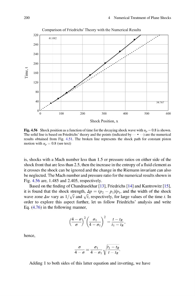
be neglected. The Mach number and pressure ratio for the numerical results shown in
Fig. 4.56 are, 1.485 and 2.405, respectively.
Based on the finding of Chandrasekhar [13], Friedrichs [14] and Kantrowitz [15],
it is found that the shock strength, Δp ¼ (p 2 À p 1 )/p 1 , and the width of the shock
wave zone Δw vary as 1=
ffi ffi
t
p
and
ffi ffi
t
p
, respectively, for large values of the time t. In
order to explore this aspect further, let us follow Friedrichs’ analysis and write
Eq. (4.76) in the following manner,
4 À σ
σ
2
σ 1
4 À σ 1
2
¼
t À t R
t 1 À t R
,
hence,
σ
4 À σ
¼
σ 1
4 À σ 1
ffiffiffiffiffiffiffiffiffiffiffiffiffi
t 1 À t R
t À t R
r
:
Adding 1 to both sides of this latter equation and inverting, we have
0
100
200
300
400
500
600
0
40
80
120
160
200
240
280
320
Comparison of Friedrichs' Theory with the Numerical Results
Shock Position, x
Time, t
34.767
61.082
Fig. 4.56 Shock position as a function of time for the decaying shock wave with u p ¼ 0.8 is shown.
The solid line is based on Friedrichs’ theory and the points (indicated by Á Á • Á Á) are the numerical
results obtained from Fig. 4.51. The broken line represents the shock path for constant piston
motion with u p ¼ 0.8 (see text)
200
4 Numerical Treatment of Plane Shocks
shock front that are less than 2.5, then the increase in the entropy of a fluid element as
it crosses the shock can be ignored and the change in the Riemann invariant can also
be neglected. The Mach number and pressure ratio for the numerical results shown in
Fig. 4.56 are, 1.485 and 2.405, respectively.
Based on the finding of Chandrasekhar [13], Friedrichs [14] and Kantrowitz [15],
it is found that the shock strength, Δp ¼ (p 2 À p 1 )/p 1 , and the width of the shock
wave zone Δw vary as 1=
ffi ffi
t
p
and
ffi ffi
t
p
, respectively, for large values of the time t. In
order to explore this aspect further, let us follow Friedrichs’ analysis and write
Eq. (4.76) in the following manner,
4 À σ
σ
2
σ 1
4 À σ 1
2
¼
t À t R
t 1 À t R
,
hence,
σ
4 À σ
¼
σ 1
4 À σ 1
ffiffiffiffiffiffiffiffiffiffiffiffiffi
t 1 À t R
t À t R
r
:
Adding 1 to both sides of this latter equation and inverting, we have
0
100
200
300
400
500
600
0
40
80
120
160
200
240
280
320
Comparison of Friedrichs' Theory with the Numerical Results
Shock Position, x
Time, t
34.767
61.082
Fig. 4.56 Shock position as a function of time for the decaying shock wave with u p ¼ 0.8 is shown.
The solid line is based on Friedrichs’ theory and the points (indicated by Á Á • Á Á) are the numerical
results obtained from Fig. 4.51. The broken line represents the shock path for constant piston
motion with u p ¼ 0.8 (see text)
200
4 Numerical Treatment of Plane Shocks