

Equations (4.76) and (4.77) are the parametric equations for the shock line and we
will use these equations for comparison with the numerical results.
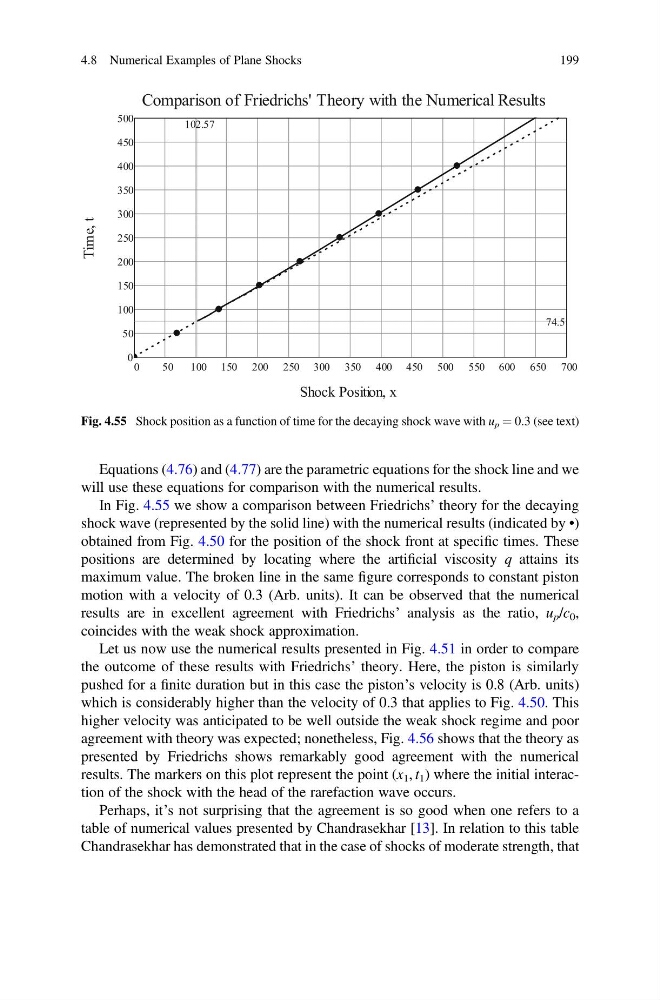
In Fig. 4.55 we show a comparison between Friedrichs’ theory for the decaying
shock wave (represented by the solid line) with the numerical results (indicated by •)
obtained from Fig. 4.50 for the position of the shock front at specific times. These
positions are determined by locating where the artificial viscosity q attains its
maximum value. The broken line in the same figure corresponds to constant piston
motion with a velocity of 0.3 (Arb. units). It can be observed that the numerical
results are in excellent agreement with Friedrichs’ analysis as the ratio, u p /c 0 ,
coincides with the weak shock approximation.
Let us now use the numerical results presented in Fig. 4.51 in order to compare
the outcome of these results with Friedrichs’ theory. Here, the piston is similarly
pushed for a finite duration but in this case the piston’s velocity is 0.8 (Arb. units)
which is considerably higher than the velocity of 0.3 that applies to Fig. 4.50. This
higher velocity was anticipated to be well outside the weak shock regime and poor
agreement with theory was expected; nonetheless, Fig. 4.56 shows that the theory as
presented by Friedrichs shows remarkably good agreement with the numerical
results. The markers on this plot represent the point (x 1 , t 1 ) where the initial interaction of the shock with the head of the rarefaction wave occurs.
Perhaps, it’s not surprising that the agreement is so good when one refers to a
table of numerical values presented by Chandrasekhar [13]. In relation to this table
Chandrasekhar has demonstrated that in the case of shocks of moderate strength, that
Fig. 4.55 Shock position as a function of time for the decaying shock wave with u p ¼ 0.3 (see text)
4.8 Numerical Examples of Plane Shocks
199
will use these equations for comparison with the numerical results.
In Fig. 4.55 we show a comparison between Friedrichs’ theory for the decaying
shock wave (represented by the solid line) with the numerical results (indicated by •)
obtained from Fig. 4.50 for the position of the shock front at specific times. These
positions are determined by locating where the artificial viscosity q attains its
maximum value. The broken line in the same figure corresponds to constant piston
motion with a velocity of 0.3 (Arb. units). It can be observed that the numerical
results are in excellent agreement with Friedrichs’ analysis as the ratio, u p /c 0 ,
coincides with the weak shock approximation.
Let us now use the numerical results presented in Fig. 4.51 in order to compare
the outcome of these results with Friedrichs’ theory. Here, the piston is similarly
pushed for a finite duration but in this case the piston’s velocity is 0.8 (Arb. units)
which is considerably higher than the velocity of 0.3 that applies to Fig. 4.50. This
higher velocity was anticipated to be well outside the weak shock regime and poor
agreement with theory was expected; nonetheless, Fig. 4.56 shows that the theory as
presented by Friedrichs shows remarkably good agreement with the numerical
results. The markers on this plot represent the point (x 1 , t 1 ) where the initial interaction of the shock with the head of the rarefaction wave occurs.
Perhaps, it’s not surprising that the agreement is so good when one refers to a
table of numerical values presented by Chandrasekhar [13]. In relation to this table
Chandrasekhar has demonstrated that in the case of shocks of moderate strength, that
Fig. 4.55 Shock position as a function of time for the decaying shock wave with u p ¼ 0.3 (see text)
4.8 Numerical Examples of Plane Shocks
199