

that depicted in Fig. 2.3. For the numerical procedure we will use the following
parameters; γ ¼ 1.4, κ ¼ 1.2, Δx ¼ 1.0, Δt ¼ 0.1 and unity values for the ambient
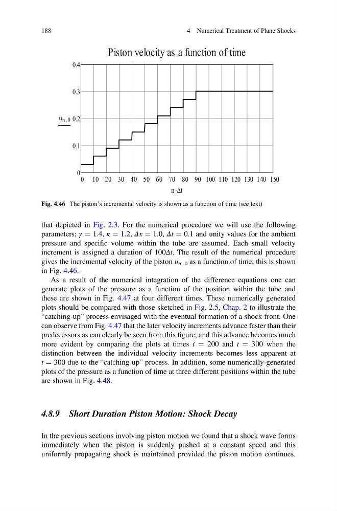
pressure and specific volume within the tube are assumed. Each small velocity
increment is assigned a duration of 100Δt. The result of the numerical procedure
gives the incremental velocity of the piston u n, 0 as a function of time; this is shown
in Fig. 4.46.
As a result of the numerical integration of the difference equations one can
generate plots of the pressure as a function of the position within the tube and
these are shown in Fig. 4.47 at four different times. These numerically generated
plots should be compared with those sketched in Fig. 2.5, Chap. 2 to illustrate the
“catching-up” process envisaged with the eventual formation of a shock front. One
can observe from Fig. 4.47 that the later velocity increments advance faster than their
predecessors as can clearly be seen from this figure, and this advance becomes much
more evident by comparing the plots at times t ¼ 200 and t ¼ 300 when the
distinction between the individual velocity increments becomes less apparent at
t ¼ 300 due to the “catching-up” process. In addition, some numerically-generated
plots of the pressure as a function of time at three different positions within the tube
are shown in Fig. 4.48.
4.8.9 Short Duration Piston Motion: Shock Decay
In the previous sections involving piston motion we found that a shock wave forms
immediately when the piston is suddenly pushed at a constant speed and this
uniformly propagating shock is maintained provided the piston motion continues.
Fig. 4.46 The piston’s incremental velocity is shown as a function of time (see text)
188
4 Numerical Treatment of Plane Shocks
parameters; γ ¼ 1.4, κ ¼ 1.2, Δx ¼ 1.0, Δt ¼ 0.1 and unity values for the ambient
pressure and specific volume within the tube are assumed. Each small velocity
increment is assigned a duration of 100Δt. The result of the numerical procedure
gives the incremental velocity of the piston u n, 0 as a function of time; this is shown
in Fig. 4.46.
As a result of the numerical integration of the difference equations one can
generate plots of the pressure as a function of the position within the tube and
these are shown in Fig. 4.47 at four different times. These numerically generated
plots should be compared with those sketched in Fig. 2.5, Chap. 2 to illustrate the
“catching-up” process envisaged with the eventual formation of a shock front. One
can observe from Fig. 4.47 that the later velocity increments advance faster than their
predecessors as can clearly be seen from this figure, and this advance becomes much
more evident by comparing the plots at times t ¼ 200 and t ¼ 300 when the
distinction between the individual velocity increments becomes less apparent at
t ¼ 300 due to the “catching-up” process. In addition, some numerically-generated
plots of the pressure as a function of time at three different positions within the tube
are shown in Fig. 4.48.
4.8.9 Short Duration Piston Motion: Shock Decay
In the previous sections involving piston motion we found that a shock wave forms
immediately when the piston is suddenly pushed at a constant speed and this
uniformly propagating shock is maintained provided the piston motion continues.
Fig. 4.46 The piston’s incremental velocity is shown as a function of time (see text)
188
4 Numerical Treatment of Plane Shocks