

Multiplying this latter equation by Sin 2m þ 1
ð
Þ
πc 0 t
2L
Â
Ã
and performing the integration in the usual manner we obtain the following equation for Δu(x, t);
Δu x, t
ð Þ ¼ 0:0003
X 1
n¼0
4=π
ð
Þ
2n þ 1
!
Cos 2n þ 1
ð
Þ
πx
2L
h
i
Sin 2n þ 1
ð
Þ
πc 0 t
2L
h
i
:
ð4:62Þ
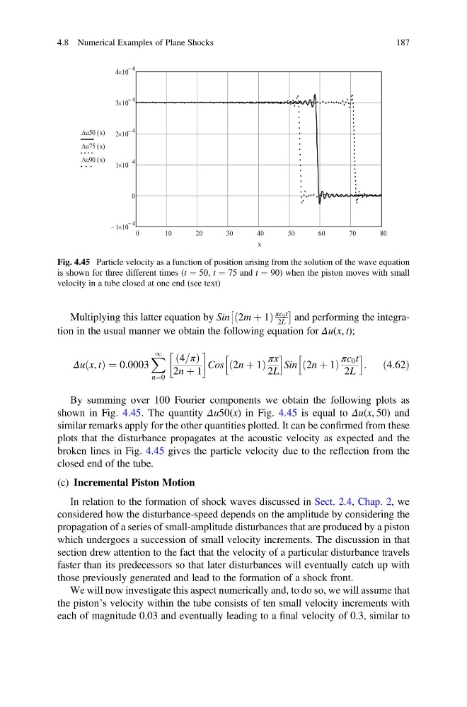
By summing over 100 Fourier components we obtain the following plots as
shown in Fig. 4.45. The quantity Δu50(x) in Fig. 4.45 is equal to Δu(x, 50) and
similar remarks apply for the other quantities plotted. It can be confirmed from these
plots that the disturbance propagates at the acoustic velocity as expected and the
broken lines in Fig. 4.45 gives the particle velocity due to the reflection from the
closed end of the tube.
(c) Incremental Piston Motion
In relation to the formation of shock waves discussed in Sect. 2.4, Chap. 2, we
considered how the disturbance-speed depends on the amplitude by considering the
propagation of a series of small-amplitude disturbances that are produced by a piston
which undergoes a succession of small velocity increments. The discussion in that
section drew attention to the fact that the velocity of a particular disturbance travels
faster than its predecessors so that later disturbances will eventually catch up with
those previously generated and lead to the formation of a shock front.
We will now investigate this aspect numerically and, to do so, we will assume that
the piston’s velocity within the tube consists of ten small velocity increments with
each of magnitude 0.03 and eventually leading to a final velocity of 0.3, similar to
Fig. 4.45 Particle velocity as a function of position arising from the solution of the wave equation
is shown for three different times (t ¼ 50, t ¼ 75 and t ¼ 90) when the piston moves with small
velocity in a tube closed at one end (see text)
4.8 Numerical Examples of Plane Shocks
187
ð
Þ
πc 0 t
2L
Â
Ã
and performing the integration in the usual manner we obtain the following equation for Δu(x, t);
Δu x, t
ð Þ ¼ 0:0003
X 1
n¼0
4=π
ð
Þ
2n þ 1
!
Cos 2n þ 1
ð
Þ
πx
2L
h
i
Sin 2n þ 1
ð
Þ
πc 0 t
2L
h
i
:
ð4:62Þ
By summing over 100 Fourier components we obtain the following plots as
shown in Fig. 4.45. The quantity Δu50(x) in Fig. 4.45 is equal to Δu(x, 50) and
similar remarks apply for the other quantities plotted. It can be confirmed from these
plots that the disturbance propagates at the acoustic velocity as expected and the
broken lines in Fig. 4.45 gives the particle velocity due to the reflection from the
closed end of the tube.
(c) Incremental Piston Motion
In relation to the formation of shock waves discussed in Sect. 2.4, Chap. 2, we
considered how the disturbance-speed depends on the amplitude by considering the
propagation of a series of small-amplitude disturbances that are produced by a piston
which undergoes a succession of small velocity increments. The discussion in that
section drew attention to the fact that the velocity of a particular disturbance travels
faster than its predecessors so that later disturbances will eventually catch up with
those previously generated and lead to the formation of a shock front.
We will now investigate this aspect numerically and, to do so, we will assume that
the piston’s velocity within the tube consists of ten small velocity increments with
each of magnitude 0.03 and eventually leading to a final velocity of 0.3, similar to
Fig. 4.45 Particle velocity as a function of position arising from the solution of the wave equation
is shown for three different times (t ¼ 50, t ¼ 75 and t ¼ 90) when the piston moves with small
velocity in a tube closed at one end (see text)
4.8 Numerical Examples of Plane Shocks
187