

which, as expected, is in accordance with the speed of the piston motion. The
velocity of the incident shock wave is estimated to be
U i ¼
140Δx
41
¼ 1:366,
which is in good agreement with the value already determined from Figs. 4.17, 4.18, 4.19 and
4.20. One can also see that this fluid element’s velocity is suddenly reduced to zero when
impacted by the reflected shock, and this is in accordance with the remarks made at the
beginning of Sect. 3.11. Further confirmation of these assertions is presented in the numerical
plot of u n, 140 versus nΔt which is also shown in Fig. 4.24.
4.8.5 The Numerical Value of κ for the Artificial Viscosity
In the previous numerical examples we have taken κ to have a value close to unity in
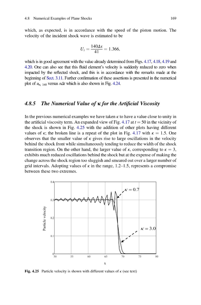
the artificial viscosity term. An expanded view of Fig. 4.17 at t ¼ 50 in the vicinity of
the shock is shown in Fig. 4.25 with the addition of other plots having different
values of κ; the broken line is a repeat of the plot in Fig. 4.17 with κ ¼ 1.5. One
observes that the smaller value of κ gives rise to large oscillations in the velocity
behind the shock front while simultaneously tending to reduce the width of the shock
transition region. On the other hand, the larger value of κ, corresponding to κ ¼ 3,
exhibits much reduced oscillations behind the shock but at the expense of making the
change across the shock region too sluggish and smeared out over a larger number of
grid intervals. Adopting values of κ in the range, 1.2–1.5, represents a compromise
between these two extremes.
Fig. 4.25 Particle velocity is shown with different values of κ (see text)
4.8 Numerical Examples of Plane Shocks
169
velocity of the incident shock wave is estimated to be
U i ¼
140Δx
41
¼ 1:366,
which is in good agreement with the value already determined from Figs. 4.17, 4.18, 4.19 and
4.20. One can also see that this fluid element’s velocity is suddenly reduced to zero when
impacted by the reflected shock, and this is in accordance with the remarks made at the
beginning of Sect. 3.11. Further confirmation of these assertions is presented in the numerical
plot of u n, 140 versus nΔt which is also shown in Fig. 4.24.
4.8.5 The Numerical Value of κ for the Artificial Viscosity
In the previous numerical examples we have taken κ to have a value close to unity in
the artificial viscosity term. An expanded view of Fig. 4.17 at t ¼ 50 in the vicinity of
the shock is shown in Fig. 4.25 with the addition of other plots having different
values of κ; the broken line is a repeat of the plot in Fig. 4.17 with κ ¼ 1.5. One
observes that the smaller value of κ gives rise to large oscillations in the velocity
behind the shock front while simultaneously tending to reduce the width of the shock
transition region. On the other hand, the larger value of κ, corresponding to κ ¼ 3,
exhibits much reduced oscillations behind the shock but at the expense of making the
change across the shock region too sluggish and smeared out over a larger number of
grid intervals. Adopting values of κ in the range, 1.2–1.5, represents a compromise
between these two extremes.
Fig. 4.25 Particle velocity is shown with different values of κ (see text)
4.8 Numerical Examples of Plane Shocks
169