

suddenly pushed into the pipe at t ¼ 0 at a constant speed u P . A shock wave is
formed immediately as the piston begins to move; initially, the position of the piston
and the shock front coincide but at later times the shock front races ahead of the
piston. The objective here is to determine the subsequent motion of the shock wave
and the associated pressure and density jumps across the shock.
The following values were chosen for the numerical procedure; Δx ¼ 0.1,
Δt ¼ 0.01, J ¼ 500, N ¼ 1000, p(x, 0) ¼ 1, υ(x, 0) ¼ 1, γ ¼ 1.4, piston velocity of
u p (0, t) ¼ 0.3 and κ in the artificial viscosity term was taken as 1.2.
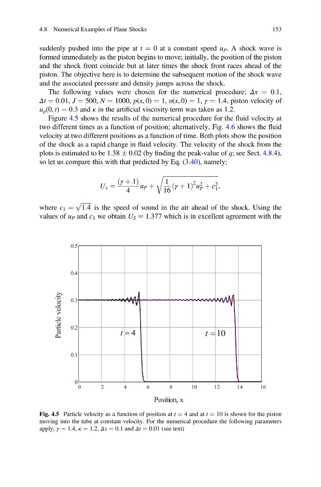
Figure 4.5 shows the results of the numerical procedure for the fluid velocity at
two different times as a function of position; alternatively, Fig. 4.6 shows the fluid
velocity at two different positions as a function of time. Both plots show the position
of the shock as a rapid change in fluid velocity. The velocity of the shock from the
plots is estimated to be 1.38 Æ 0.02 (by finding the peak-value of q; see Sect. 4.8.4),
so let us compare this with that predicted by Eq. (3.40), namely;
U s ¼
γ þ 1
ð
Þ
4
u P þ
ffiffiffiffiffiffiffiffiffiffiffiffiffiffiffiffiffiffiffiffiffiffiffiffiffiffiffiffiffiffiffiffiffiffiffiffi ffi
1
16
γ þ 1
ð
Þ
2 u 2
P þ c 2
1
r
,
where c 1 ¼
ffiffiffiffiffiffi ffi
1:4
p
is the speed of sound in the air ahead of the shock. Using the
values of u P and c 1 we obtain U S ¼ 1.377 which is in excellent agreement with the
Fig. 4.5 Particle velocity as a function of position at t ¼ 4 and at t ¼ 10 is shown for the piston
moving into the tube at constant velocity. For the numerical procedure the following parameters
apply; γ ¼ 1.4, κ ¼ 1.2, Δx ¼ 0.1 and Δt ¼ 0.01 (see text)
4.8 Numerical Examples of Plane Shocks
153
formed immediately as the piston begins to move; initially, the position of the piston
and the shock front coincide but at later times the shock front races ahead of the
piston. The objective here is to determine the subsequent motion of the shock wave
and the associated pressure and density jumps across the shock.
The following values were chosen for the numerical procedure; Δx ¼ 0.1,
Δt ¼ 0.01, J ¼ 500, N ¼ 1000, p(x, 0) ¼ 1, υ(x, 0) ¼ 1, γ ¼ 1.4, piston velocity of
u p (0, t) ¼ 0.3 and κ in the artificial viscosity term was taken as 1.2.
Figure 4.5 shows the results of the numerical procedure for the fluid velocity at
two different times as a function of position; alternatively, Fig. 4.6 shows the fluid
velocity at two different positions as a function of time. Both plots show the position
of the shock as a rapid change in fluid velocity. The velocity of the shock from the
plots is estimated to be 1.38 Æ 0.02 (by finding the peak-value of q; see Sect. 4.8.4),
so let us compare this with that predicted by Eq. (3.40), namely;
U s ¼
γ þ 1
ð
Þ
4
u P þ
ffiffiffiffiffiffiffiffiffiffiffiffiffiffiffiffiffiffiffiffiffiffiffiffiffiffiffiffiffiffiffiffiffiffiffiffi ffi
1
16
γ þ 1
ð
Þ
2 u 2
P þ c 2
1
r
,
where c 1 ¼
ffiffiffiffiffiffi ffi
1:4
p
is the speed of sound in the air ahead of the shock. Using the
values of u P and c 1 we obtain U S ¼ 1.377 which is in excellent agreement with the
Fig. 4.5 Particle velocity as a function of position at t ¼ 4 and at t ¼ 10 is shown for the piston
moving into the tube at constant velocity. For the numerical procedure the following parameters
apply; γ ¼ 1.4, κ ¼ 1.2, Δx ¼ 0.1 and Δt ¼ 0.01 (see text)
4.8 Numerical Examples of Plane Shocks
153