

value above. The pressure and density jumps across the shock are given by
Eqs. (3.25) and (3.28), namely,
p 2
p 1
¼ 1 þ
2γ
γ þ 1
M
2
1 À 1
À
Á
and
ρ 2
ρ 1
¼
γ þ 1
ð
ÞM
2
1
γ À 1
ð
ÞM
2
1 þ 2
Â
à ,
respectively, where M 1 ¼ U S /c 1 . Accordingly, these equations give p 2 ¼ 1.413 and
ρ 2 ¼ 1.278. The corresponding plots of the pressure and density are shown in
Figs. 4.7 and 4.8, respectively, and a numerical estimate of these jumps yields
p 2 ¼ 1.413 Æ 0.001 and ρ 2 ¼ 1.278 Æ 0.001 for the pressure and density in the
relatively flat portions behind the shock.
Plots of the fluid velocity are shown in Figs. 4.9 and 4.10 where the step size is
reduced by an order of magnitude. One can observe that the shock front displays a
sharper transition with much reduced oscillations. An expanded plot in the vicinity
of the shock is shown in Fig. 4.11. It can be seen that the width of the shock front is
approximately four to five spatial (or time) increments.
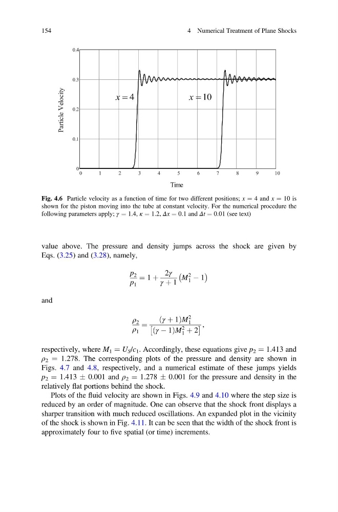
Fig. 4.6 Particle velocity as a function of time for two different positions; x ¼ 4 and x ¼ 10 is
shown for the piston moving into the tube at constant velocity. For the numerical procedure the
following parameters apply; γ ¼ 1.4, κ ¼ 1.2, Δx ¼ 0.1 and Δt ¼ 0.01 (see text)
154
4 Numerical Treatment of Plane Shocks
Eqs. (3.25) and (3.28), namely,
p 2
p 1
¼ 1 þ
2γ
γ þ 1
M
2
1 À 1
À
Á
and
ρ 2
ρ 1
¼
γ þ 1
ð
ÞM
2
1
γ À 1
ð
ÞM
2
1 þ 2
Â
à ,
respectively, where M 1 ¼ U S /c 1 . Accordingly, these equations give p 2 ¼ 1.413 and
ρ 2 ¼ 1.278. The corresponding plots of the pressure and density are shown in
Figs. 4.7 and 4.8, respectively, and a numerical estimate of these jumps yields
p 2 ¼ 1.413 Æ 0.001 and ρ 2 ¼ 1.278 Æ 0.001 for the pressure and density in the
relatively flat portions behind the shock.
Plots of the fluid velocity are shown in Figs. 4.9 and 4.10 where the step size is
reduced by an order of magnitude. One can observe that the shock front displays a
sharper transition with much reduced oscillations. An expanded plot in the vicinity
of the shock is shown in Fig. 4.11. It can be seen that the width of the shock front is
approximately four to five spatial (or time) increments.
Fig. 4.6 Particle velocity as a function of time for two different positions; x ¼ 4 and x ¼ 10 is
shown for the piston moving into the tube at constant velocity. For the numerical procedure the
following parameters apply; γ ¼ 1.4, κ ¼ 1.2, Δx ¼ 0.1 and Δt ¼ 0.01 (see text)
154
4 Numerical Treatment of Plane Shocks