

4.7 Grid Spacing
We now come to the question of the choice of grid spacing Δx in order to identify the
position of the shocks with some accuracy [8]. Recalling from our previous discussion that the typical shock thickness is the order of the molecular mean-free-path l mfp ,
and it would appear essential to have the grid spacing Δx % l mfp to realistically model
fluid flow in the presence of shocks. However, having Δx % l mfp implies that the
time-step Δt must be less than l mfp /c in order to satisfy the CFL condition above,
where c is the signal propagation speed. Typically, l mfp % 10
À5 cm and this implies
that the computing time necessary to follow a specific time interval could become
prohibitive. Accordingly, the choice of grid size Δx represents a compromise
between accuracy in locating the position of the shock and the total computing
time required for any specific application. With artificial viscosity included we will
see in due course that the shock acquires a thickness of the order of a few Δx.
4.8 Numerical Examples of Plane Shocks
In the following sections we will investigate the numerical solution to several
examples of plane shock waves.
4.8.1 Piston Generated Shock Wave
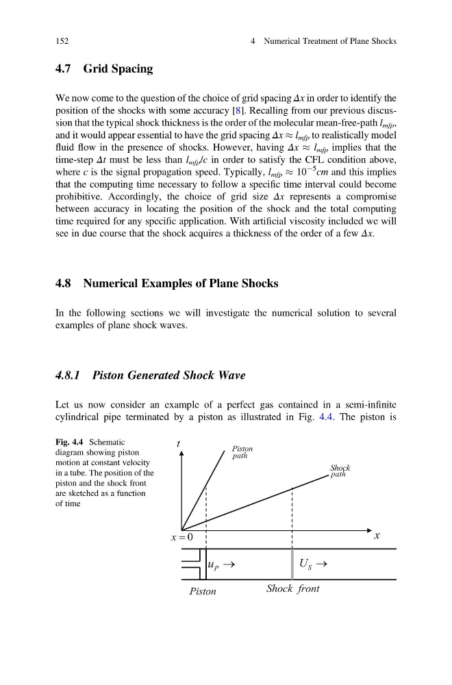
Let us now consider an example of a perfect gas contained in a semi-infinite
cylindrical pipe terminated by a piston as illustrated in Fig. 4.4. The piston is
Fig. 4.4 Schematic
diagram showing piston
motion at constant velocity
in a tube. The position of the
piston and the shock front
are sketched as a function
of time
152
4 Numerical Treatment of Plane Shocks
We now come to the question of the choice of grid spacing Δx in order to identify the
position of the shocks with some accuracy [8]. Recalling from our previous discussion that the typical shock thickness is the order of the molecular mean-free-path l mfp ,
and it would appear essential to have the grid spacing Δx % l mfp to realistically model
fluid flow in the presence of shocks. However, having Δx % l mfp implies that the
time-step Δt must be less than l mfp /c in order to satisfy the CFL condition above,
where c is the signal propagation speed. Typically, l mfp % 10
À5 cm and this implies
that the computing time necessary to follow a specific time interval could become
prohibitive. Accordingly, the choice of grid size Δx represents a compromise
between accuracy in locating the position of the shock and the total computing
time required for any specific application. With artificial viscosity included we will
see in due course that the shock acquires a thickness of the order of a few Δx.
4.8 Numerical Examples of Plane Shocks
In the following sections we will investigate the numerical solution to several
examples of plane shock waves.
4.8.1 Piston Generated Shock Wave
Let us now consider an example of a perfect gas contained in a semi-infinite
cylindrical pipe terminated by a piston as illustrated in Fig. 4.4. The piston is
Fig. 4.4 Schematic
diagram showing piston
motion at constant velocity
in a tube. The position of the
piston and the shock front
are sketched as a function
of time
152
4 Numerical Treatment of Plane Shocks